Educational Inequality

Educational Inequality in LA Unified School District and the LCFF

Schools often boast of their students' achievements, but does this reflect well on the school itself, or only the students? After all, schools with more money or prestige can recruit high achieving students. So when the high test scores come in, does that reflect recruitment success or success on the parts of teachers and school administration?

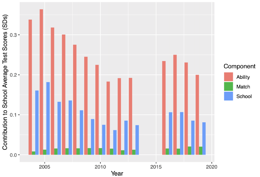
With twenty years of data and over a million students' demographics grades and test scores, student achievement can be decomposed into three components:

the student’s ability
the school’s ability to educate students
an idiosyncratic “match effect”

Everyone has a story of a particular teacher who for better or for worse, significantly changed the course of their academic career. If you had happened to be assigned geographically to a different high school, that new school wouldn’t have offered you the chance (or misfortune) of interacting with that particular teacher. This is what is meant by idiosyncratic match effects.

The Model

Suppose there are J_t schools in each time period t and I_t students for t= 1,…,T. We model potential outcomes of students as:

Y_ij = α_j + β_j^T X_i + ε

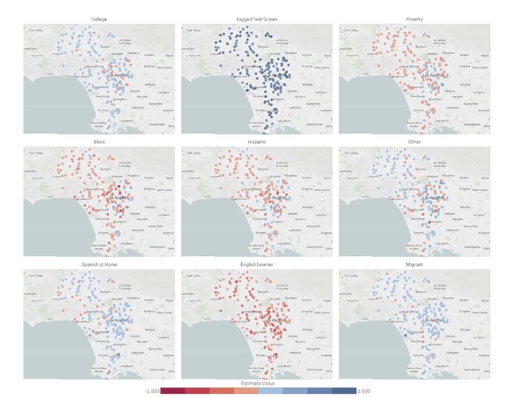
where α_j is a school effect, X_i are student i’s characteristics, and u_ij is a school-specific idiosyncratic factor. Note that this model allows for both vertical differentiation—through the α_j– and horizontal differentiation—through the β_j^T X_i term. Building on this model, we now proceed to decompose potential achievement into the three components discussed above.

First, we define student ability A_i as the average of student i’s potential outcome across all schools j

A_i = J^-1 ∑ Y_ij = α + β^T X_i + ε_i

With a notion of ability, we can express potential outcomes as

Y_ij = A_i - A_i + α_j + β_j^T X_i + ε_i

Y_ij = A_i + (α_j-α) + (β_j-β)^T X_i + ε_ij - ε_i

Y_ij = Ability + ATE_j + M_ij (Match Effect)

which depends on student ability, the average treatment effect of school j ATE_j, and i-j match effect M_ij. A_i captures how well a student does, on average, independent of the school they attend. ATE_j captures how much school j improves its student’s test scores above and beyond the average school in the district. M_ij captures the prevalence of sorting but we are agnostic about its sign. If M_ij is positive then students sort into schools that improve their outcomes relative to the average school e.g. some schools are particularly effective educating impoverished students.(A school j that met this criteria would have (β_j^Poor - β^Poor )>0 indicating poor students will yield positive returns to attending school j compared to the average school.)

With the decomposition of potential outcomes above, we can express school-level average outcomes as a function of the three components. Specifically, average test scores of school j is

E[Y_ij | j(i) = j ] = E[A_i | j(i) = j] + ATE_j + E[M_ij | j(i) = j]

E[Y_ij | j(i) = j ] = Q_j + ATE_j + M_j

where Q_j represents the average ability of students attending school j, ATE_j is defined above, and M_j captures the average match effect of students attending school j. Returning to our motivating example, a school that attracts high achieving students with be a school with high Q_j but not necessarily high ATE_j. The ATE_j, in contrast, captures the average effect of attending school j relative to the average school in the district. Thus, a school with ATE_j>0 is above average in terms of improving the academic achievement of its students, while a school with ATE_j<0 is below average. Regardless of the value of ATE_j, it is a more adequate notion of school quality since it represents the average impact of school j on its students' achievement, regardless of the students' underlying ability.

It is important to emphasize that publicly available data on school achievement will report E[Y_ij | j(i) = j ] and implicitly combine the three components we defined. Therefore, some schools may appear to be high performing because they attract students with high average ability Q_j but have low ATE_j. A school with these characteristics would not improve the academic trajectory of its students, but appear to be high-performing due to the fact that the average student would do well regardless of the school they attended. Thus, when discussing within-district inequality we’ll refer to differences in the ATE_j over time as opposed to differences in E[Y_ij | j(i) = j ].

The LCFF

In 2012 Governor Jerry Brown proposed the Local Control Funding Formula (LCFF) with a threefold aim: requiring school districts to focus on eight key areas to help students succeed, providing extra funding for students with greater challenges, and giving school districts more flexibility in spending money to improve schools. The measure pledged 18 billion dollars to California schools over 6 years. Furthermore, the LCFF included the Local Control and Accountability Plan (LCAP), wherein school districts were meant to engage the local community in specific, measurable, and timely implementation of the LCFF.

Despite the LCFF’s aims, a report by Education Trust West found that although poorer districts received on average more funding, in some schools, inequality gaps have widened. Critics have also argued that basing the funding on average daily attendance (ADA) instead of total enrollment, disproportionately affects low-income communities, which were the orig- inal proposed targets of the funding. Others have raised concerns that the LCFF is a “dump truck” solution, i.e. money goes to the districts or schools without ensuring it benefits the specific students it intended to, as opposed to a “backpack” model, where the students whose attendance merits the funding also receive the proportional benefit.

Results

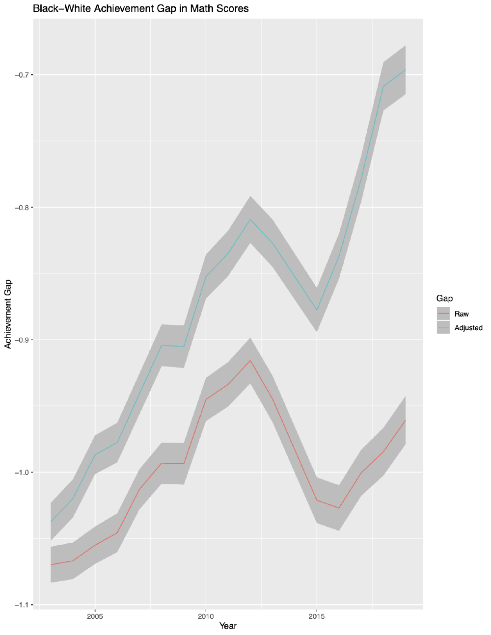
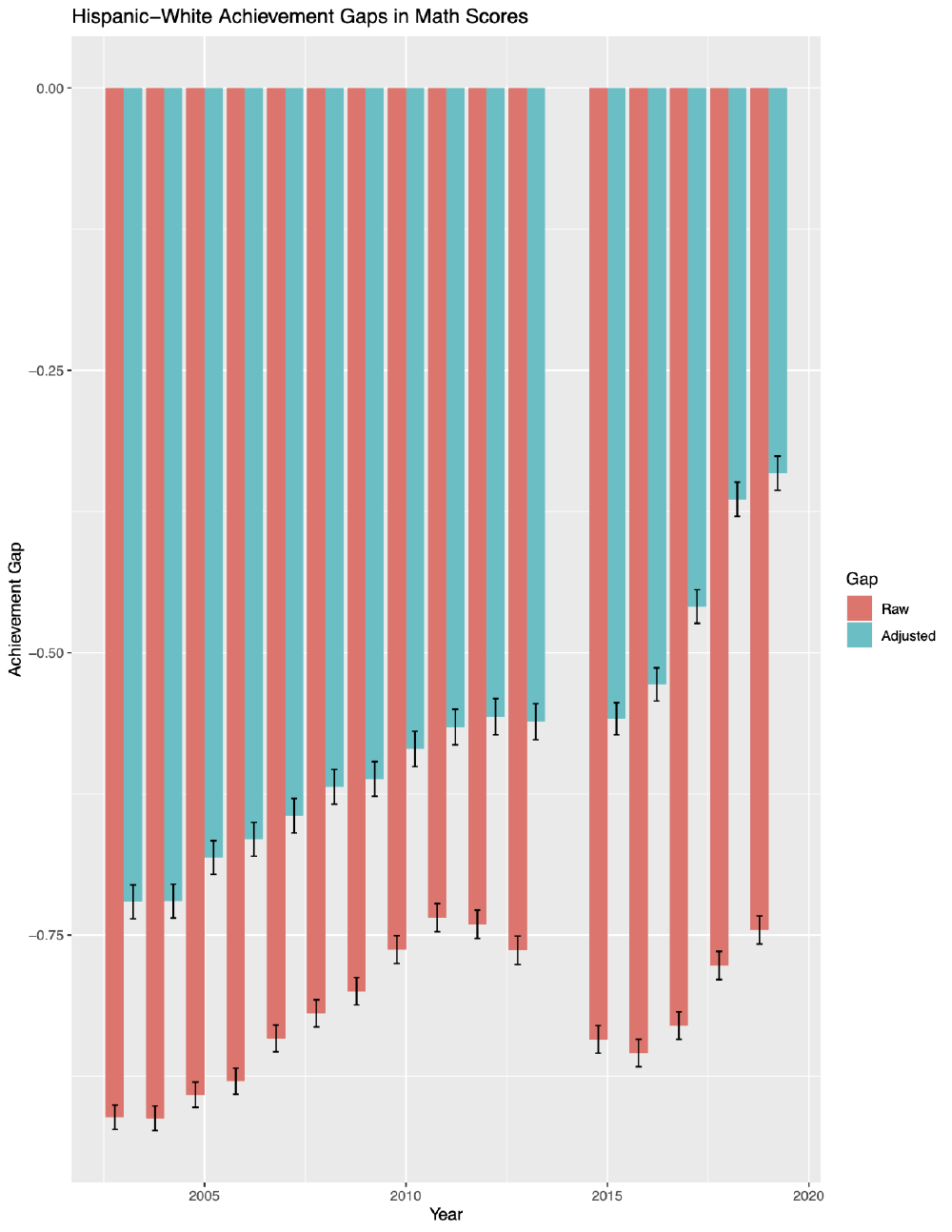
Through our novel decomposition of student test scores, we find not only disparities in student outcomes between racial groups, but value added within-school differences as well. Furthermore, we find different results than the Education Trust West study in that the LCFF decreased inequality, and suggests an upward trend moving into 2019-2020. Despite finding substantial mismanagement of allocation and disbursal of the funds, we’re hopeful that the full effects of the funding for future reductions in inequality will be seen in years to come.