11 Cluster-Robust Standard Errors
Correcting Inference When Observations Are Not Independent
When observations share a common group (classroom, firm, region), residuals within the group are correlated. Ignoring this correlation makes standard errors too small and rejection rates too high. Cluster-robust standard errors fix inference without changing point estimates.
This page assumes familiarity with panel data structure and pooled OLS and the fixed effects intuition. You should be comfortable with the composite error \(v_{ij} = u_j + e_{ij}\) and understand why pooled OLS ignores group-level heterogeneity.
11.1 The Problem: Correlated Residuals
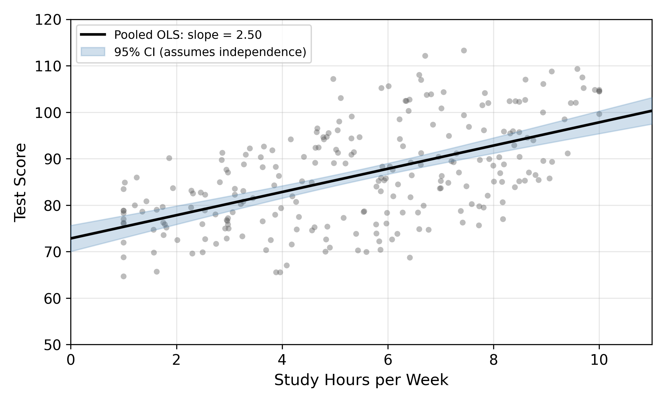
A school district tracks study hours and test scores for 240 students. We start with the simplest possible model, ignoring any group structure:
\[ \text{Score}_{ij} = \beta_0 + \beta_1 \, \text{Hours}_{ij} + \varepsilon_{ij} \tag{11.1}\]
OLS treats all 240 students as independent observations. One intercept, one slope, one error term. The standard assumption is that \(\varepsilon_i\) and \(\varepsilon_k\) are uncorrelated for all \(i \neq k\).
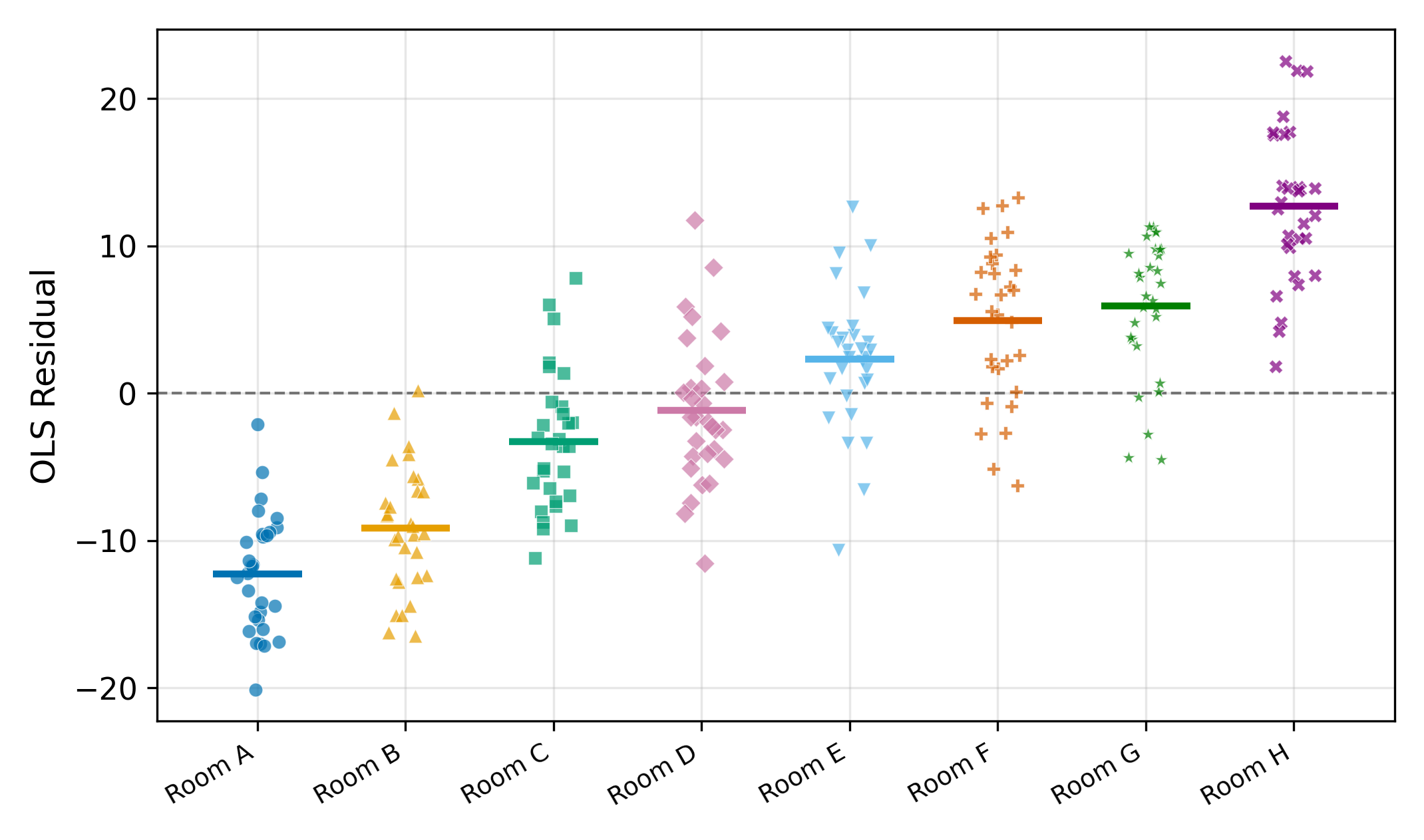
But these 240 students come from 8 different classrooms. Students in the same classroom share a teacher, a curriculum, grading norms, and peer effects. All of these unobserved factors enter the error term. When we write the model with proper subscripts (student \(i\) in classroom \(j\)), the error has two parts:
\[ v_{ij} = u_j + e_{ij} \tag{11.2}\]
- \(u_j\) = classroom-level shock (shared by all students in classroom \(j\))
- \(e_{ij}\) = idiosyncratic student-level noise (independent across students)
Analogy: surveying 240 people about a policy. If they come from 240 different households, each response is independent. If they come from 8 large families (30 per family), family members think alike and you really have about 8 independent opinions.
What pooled OLS calls \(\varepsilon_i\) is really this composite error \(v_{ij}\). Two students \(i\) and \(k\) in the same classroom \(j\) share the same \(u_j\), so their composite errors are correlated even when \(e_{ij}\) and \(e_{kj}\) are independent.
11.2 The Consequences: Standard Errors Are Too Small
The within-cluster correlation has a clean formula. For two students \(i\) and \(k\) in the same classroom \(j\):
\[ \text{Corr}(v_{ij}, v_{kj}) = \rho = \frac{\sigma_u^2}{\sigma_u^2 + \sigma_e^2} \tag{11.3}\]
This ratio \(\rho\) is called the intraclass correlation (ICC). It measures what share of total error variance comes from the classroom level. In our dataset, \(\hat{\rho} \approx 0.75\).
The standard OLS variance formula for the slope is:
\[ \text{Var}(\hat{\beta}_1) = \frac{\sigma^2}{\sum_{i=1}^{n}(x_i - \bar{x})^2} \]
This formula drops all \(\text{Cov}(v_i, v_k)\) cross-terms because it assumes independence. When within-cluster errors are positively correlated, those cross-terms are positive, making the true variance larger than what OLS reports.
The effective sample size quantifies the damage:
\[ n_{\text{eff}} = \frac{n}{1 + (m - 1)\hat{\rho}} \tag{11.4}\]
where \(n\) is the total number of observations and \(m\) is the number of observations per cluster. With \(n = 240\), \(m = 30\), and \(\hat{\rho} = 0.75\):
\[ n_{\text{eff}} = \frac{240}{1 + 29 \times 0.75} \approx 11 \]
OLS thinks it has 240 independent data points. It actually has about 11.
The effective sample size formula (Equation 11.4) shows that the damage grows with both \(\rho\) (how correlated errors are) and \(m\) (how large clusters are). A small \(\rho\) with huge clusters can be just as bad as a large \(\rho\) with moderate clusters.
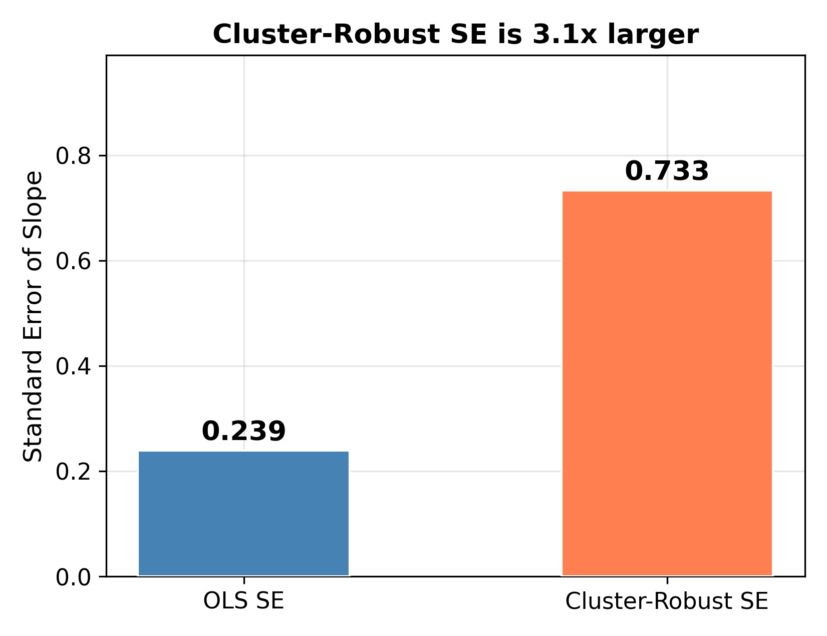
The consequences cascade through the entire inference pipeline. Same point estimate (\(\hat{\beta}_1 = 2.50\)), but the cluster-robust 95% CI is \([0.76, 4.23]\) while the OLS CI is \([2.03, 2.97]\). The cluster-robust interval is about 3.7 times wider.
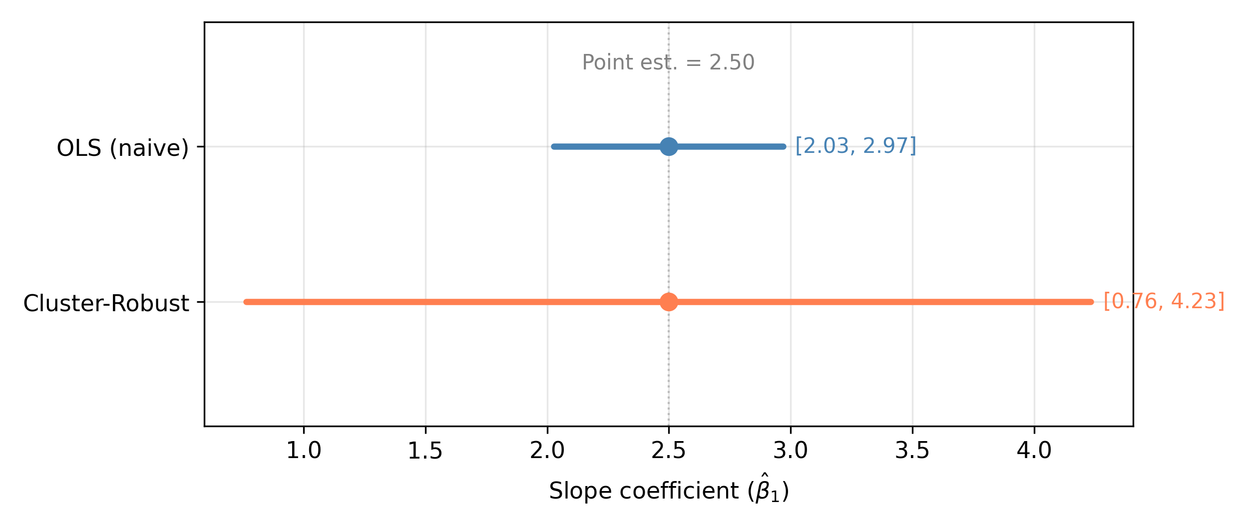
Why 3.7 times wider when the SE is only 3.1 times larger? The critical value also changes: with 8 clusters, inference uses \(t_{0.025, 7} = 2.36\) instead of \(t_{0.025, 238} = 1.97\). Fewer clusters raise the bar for significance.
\(\implies\) OLS standard errors are too small, confidence intervals are too narrow, and \(p\)-values are too small. You reject the null too often.
11.3 The Intraclass Correlation
The ICC (Equation 11.3) deserves its own discussion because it drives everything else. Two interpretations:
Correlation interpretation: \(\rho\) is the correlation between the composite errors of any two observations in the same cluster.
Variance decomposition: \(\rho\) is the fraction of total error variance that is between-group rather than within-group.
An ICC of 0.75 means 75% of total error variance is between classrooms. Only 25% is genuinely student-level noise. The classroom a student sits in dominates individual idiosyncratic factors.
When \(\rho\) is close to 1, almost all variation is between clusters. Observations within a cluster are nearly identical (from an error perspective), so adding more students to the same classroom adds very little new information. When \(\rho\) is close to 0, there’s no meaningful cluster structure and each observation is approximately independent.
When \(\rho = 0\), there is no within-cluster correlation. The composite error is essentially just \(e_{ij}\) because \(\sigma_u^2 = 0\). In that case, the effective sample size (Equation 11.4) becomes \(n_{\text{eff}} = n/(1 + 0) = n\), so all observations are independent. The cluster-robust standard error reduces to the ordinary OLS standard error. Clustering is harmless but unnecessary.
11.4 The Cluster-Robust Variance Estimator
The fix is conceptually straightforward. Instead of treating each residual as an independent draw, group residuals by cluster and allow arbitrary correlation within each cluster.
The procedure for a single regressor with \(G\) clusters:
- Run pooled OLS as usual to get \(\hat{\beta}_1\) and residuals \(\hat{e}_{ij}\).
- Group the residuals by cluster.
- For each cluster \(j\), compute the sum of residual-times-regressor products: \(S_j = \sum_{i \in \text{cluster } j} \hat{e}_{ij}(x_{ij} - \bar{x})\).
- The cluster-robust variance sums the squared cluster contributions: \(\widehat{\text{Var}}_{\text{CR}}(\hat{\beta}_1) \propto \sum_{j=1}^{G} S_j^2\).
In the standard OLS formula, each individual residual enters separately. In the cluster-robust formula, residuals within the same cluster are summed before squaring. This is what “allows arbitrary within-cluster correlation” means in practice: by summing within cluster first, positive within-cluster correlations accumulate rather than being ignored.
This is often called a “sandwich estimator” because the formula has the structure \((\text{bread})^{-1} \times \text{meat} \times (\text{bread})^{-1}\). The “bread” is the usual OLS component. The “meat” is where cluster-level sums replace individual observations.
The point estimate \(\hat{\beta}_1\) does not change. Only the standard error changes. In software:
- Stata:
reg score hours, vce(cluster classroom) - Python (statsmodels):
OLS(y, X).fit(cov_type='cluster', cov_kwds={'groups': classroom}) - R (lmtest + sandwich):
coeftest(model, vcov = vcovCL(model, cluster = ~ classroom))
11.5 Simulation: How Often Does OLS Wrongly Reject?
To see the practical damage, we simulated 1,000 datasets where the true slope is \(\beta_1 = 0\) and tested \(H_0\!: \beta_1 = 0\) at \(\alpha = 0.05\). Each dataset draws fresh classroom effects \(u_j\) from the data generating process with \(\rho = 0.75\).
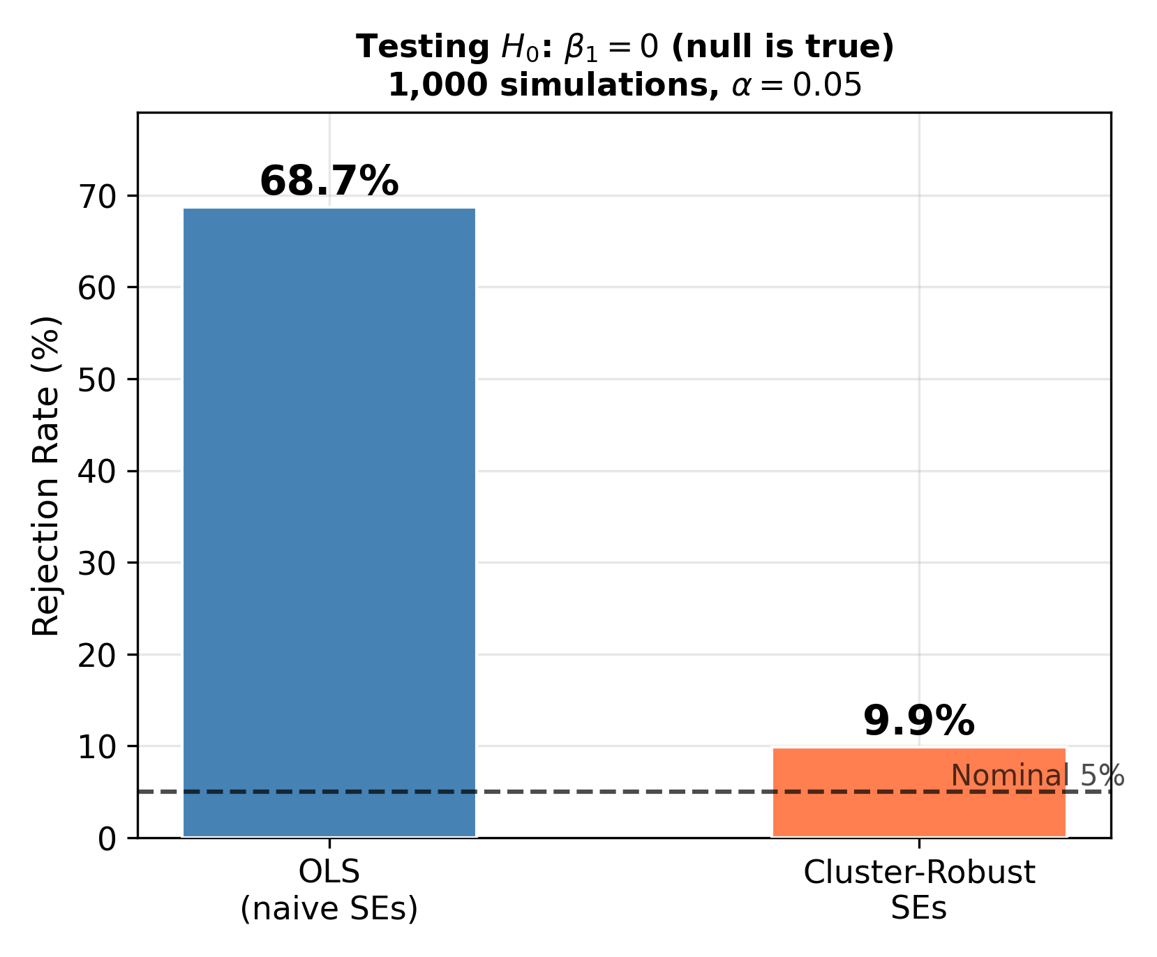
Nominal vs. actual rejection rates: a 5% test should reject a true null 5% of the time. OLS rejects at 68.7% here, meaning nearly 7 out of 10 “significant” results are false positives. With cluster-robust SEs and only 8 clusters, the rate is 9.9%. With more clusters (say 50+), cluster-robust tests get closer to the nominal 5%.
The simulation makes the stakes concrete. A researcher using naive OLS standard errors on this kind of data would “discover” statistically significant effects most of the time, even when there is nothing there.
11.6 When to Cluster
The guiding principle is: cluster at the level where treatment is assigned or where unobserved common shocks arise.
| Setting | Cluster on |
|---|---|
| Students in classrooms | Classroom |
| Workers in firms | Firm |
| State-level policy, individual data | State |
| Panel data (same person over time) | Individual |
| Patients in hospitals | Hospital |
When in doubt, cluster at the broadest plausible level. The cost of clustering when it is unnecessary is a small efficiency loss. The cost of not clustering when you should is invalid inference: wrong standard errors, wrong confidence intervals, wrong \(p\)-values.
How many clusters are enough? Cluster-robust standard errors become unreliable with fewer than about 30 clusters. In our simulation with 8 clusters, the rejection rate was 9.9% instead of the nominal 5%. With very few clusters, consider small-sample corrections or the wild cluster bootstrap (beyond the scope of this course).
It depends on where the common shocks arise. If the concern is school-level factors (principal quality, school resources, peer composition), cluster by school. If the concern is district-level factors (district funding, district policies, local labor markets), cluster by district.
The conservative choice is to cluster at the broader level (district), because district-level shocks affect all schools within the district. But with only 5 districts, you have very few clusters and inference becomes unreliable. This is the tension: broader clustering is more conservative but requires more clusters.
In practice, if you believe school-level variation is the dominant source of correlation and you have 30 schools, clustering by school gives you more clusters and more reliable standard errors. Report both and discuss the tradeoff.
11.7 What Clustering Does NOT Fix
Cluster-robust standard errors fix the standard errors, not the slope. This distinction is critical.
Suppose better-teacher classrooms also assign more study hours. The slope \(\hat{\beta}_1\) suffers from omitted variable bias because teacher quality is correlated with the regressor. Clustering makes your standard error honest about a biased slope, but it does not remove the bias.
| Clustering alone | FE + clustering | |
|---|---|---|
| SE correct? | Yes | Yes |
| Slope unbiased? | No (if OVB) | Yes |
\(\implies\) Clustering corrects inference (SEs, CIs, \(p\)-values). It does not correct estimation (the slope itself). For that, you need fixed effects. In practice, you often need both: FE to remove the bias, plus clustering on the FE residuals to get correct standard errors.
Three things clustering does not address:
Omitted variable bias. If group effects are correlated with the regressor, the point estimate is inconsistent regardless of how you compute the standard error.
Heterogeneity in slopes. Clustering assumes a common slope across all groups. If the effect of study hours differs by classroom, you need a different model.
Endogeneity from other sources. Clustering addresses error correlation, not simultaneity, measurement error, or reverse causality.
11.8 Summary
We started with 240 students, a clean regression, and a tight confidence interval. It looked precise. But the 240 students came from only 8 classrooms, and those 240 observations carried about as much independent information as 11.
| Scenario | Error structure | SE formula | Result |
|---|---|---|---|
| Independent errors | \(\text{Corr}(\varepsilon_i, \varepsilon_k) = 0\) | Standard OLS | Correct inference |
| Clustered errors, OLS SE | \(\text{Corr}(v_{ij}, v_{kj}) = \rho > 0\) | Standard OLS | SEs too small, reject too often |
| Clustered errors, CR SE | \(\text{Corr}(v_{ij}, v_{kj}) = \rho > 0\) | Cluster-robust | Correct (or approximately correct) inference |
The logic in five steps:
Pooled OLS on clustered data can give a reasonable slope estimate, but the standard errors are too small because they ignore within-cluster error correlation.
The intraclass correlation \(\rho\) (Equation 11.3) measures how much error variance is between clusters vs. within clusters. Higher \(\rho\) \(\implies\) worse SE distortion.
The effective sample size (Equation 11.4) quantifies the information loss. With \(\rho = 0.75\) and 30 students per classroom, 240 observations carry about as much information as 11.
Cluster-robust SEs fix the standard errors by allowing arbitrary within-cluster correlation. The point estimate does not change.
Clustering fixes inference, not estimation. If group effects are correlated with the regressor, you also need fixed effects to remove the bias.
Rule of thumb: if you can point to a grouping variable that might create shared unobservables, cluster on it. The downside of unnecessary clustering is small. The downside of missing it is large.
Continue to dynamic panel models to see what happens when lagged dependent variables appear as regressors. Or return to the panel data overview for the complete roadmap.