12 Dynamic Panel Models
Lagged Dependent Variables, Nickell Bias, and GMM Estimation
Many economic outcomes are persistent: GDP this year depends on GDP last year. Adding a lagged dependent variable to a panel model creates endogeneity that neither OLS nor fixed effects can solve. Arellano-Bond GMM uses lagged levels as instruments for first-differenced equations.
This page assumes familiarity with panel data models (fixed effects and random effects). See Panel Data Models for the general framework and Fixed Effects: The Intuition for the within estimator.
12.1 Persistence in Panel Data
Many economic outcomes are persistent. A country with high GDP this year will almost certainly have high GDP next year. A worker earning high wages today is unlikely to earn minimum wage tomorrow. Firm profits, trade balances, health expenditures: all exhibit strong autocorrelation.
A natural way to model this persistence is to include the lagged outcome on the right-hand side:
\[ y_{it} = \rho \, y_{i,t-1} + \beta \, x_{it} + \alpha_i + \varepsilon_{it} \tag{12.1}\]
where \(\rho\) captures the degree of persistence, \(x_{it}\) is an observed regressor, \(\alpha_i\) is an individual fixed effect, and \(\varepsilon_{it}\) is idiosyncratic error. The parameter \(\rho\) tells us how strongly the past predicts the present, after controlling for observables and unobserved heterogeneity.
When \(|\rho| < 1\), a shock to \(y_{it}\) fades over time. When \(\rho = 1\), shocks are permanent (unit root). Most panel applications assume \(|\rho| < 1\).
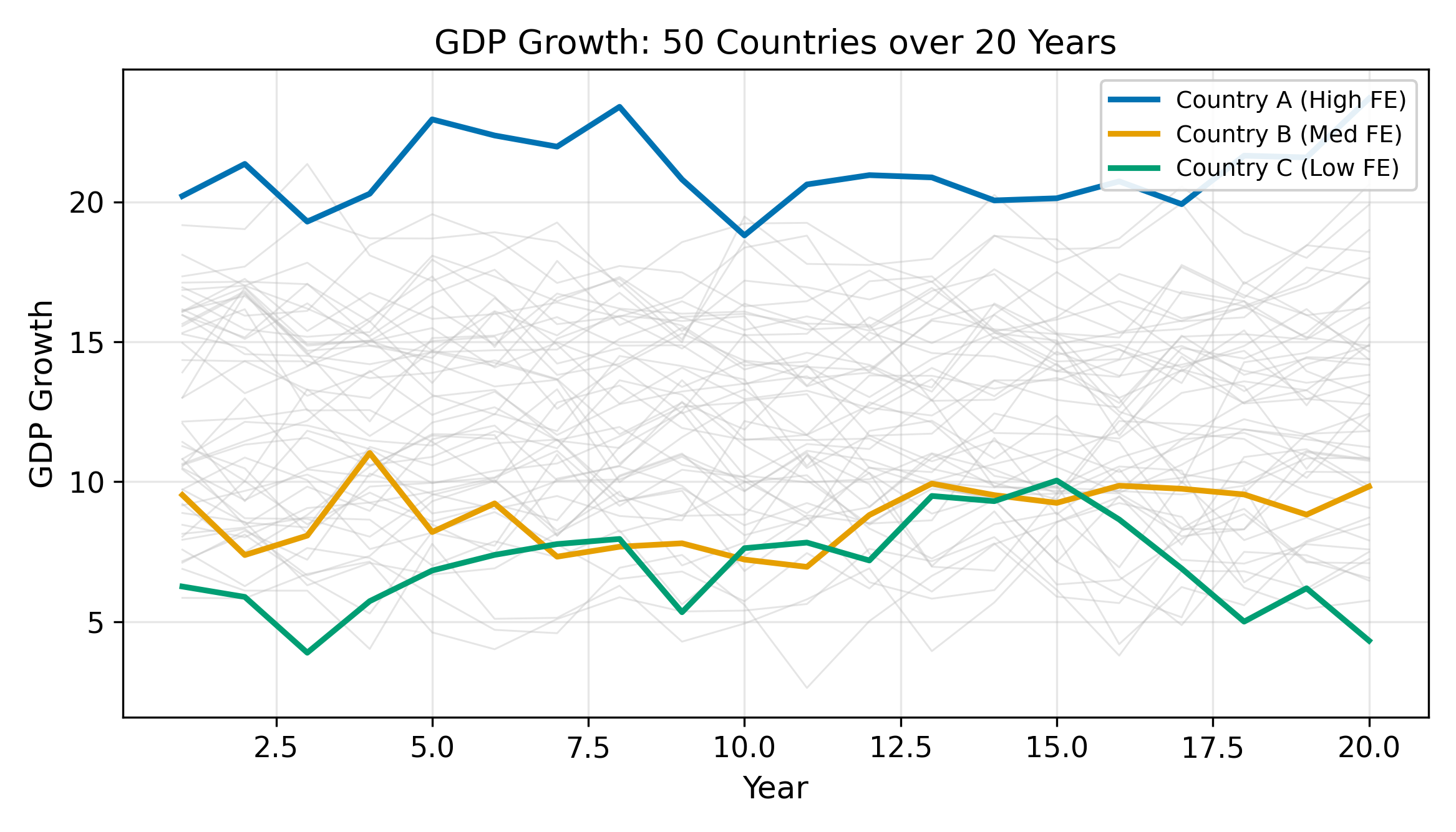
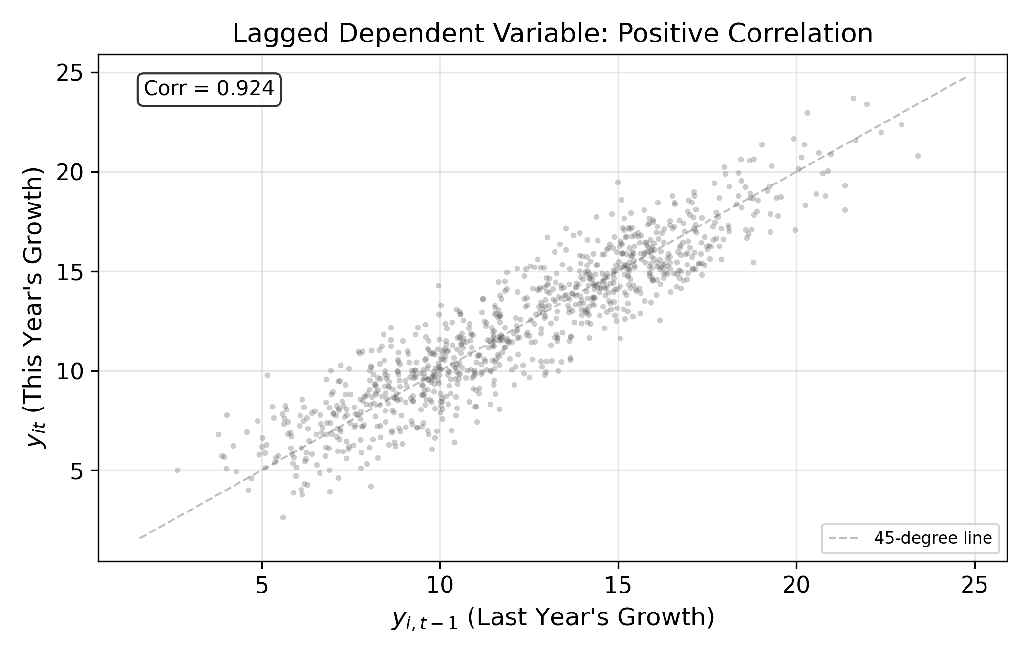
The time series plot in Figure 12.1 illustrates this persistence visually. The lagged scatter in Figure 12.2 makes the autocorrelation even more explicit: plotting \(y_{it}\) against \(y_{i,t-1}\) shows a clear positive relationship.
The question is how to estimate \(\rho\) and \(\beta\) consistently. Neither OLS nor fixed effects can do it.
12.2 Why OLS Fails
The problem is straightforward. In Equation 12.1, \(y_{i,t-1}\) depends on \(\alpha_i\) because \(\alpha_i\) enters every period’s outcome. A country with a permanently higher growth rate (\(\alpha_i\) is large) will have higher \(y_{i,t-1}\) in every period. So the lagged dependent variable and the fixed effect are positively correlated:
\[ \text{Cov}(y_{i,t-1}, \alpha_i) > 0 \]
Since \(\alpha_i\) is part of the composite error in the pooled model, this violates the OLS exogeneity condition. OLS attributes some of the permanent level shift (caused by \(\alpha_i\)) to the lagged dependent variable, inflating \(\hat{\rho}\).
\(\implies\) OLS is biased upward: it overestimates persistence.
OLS overestimates persistence because the fixed effect creates a permanent level shift that looks like autocorrelation.
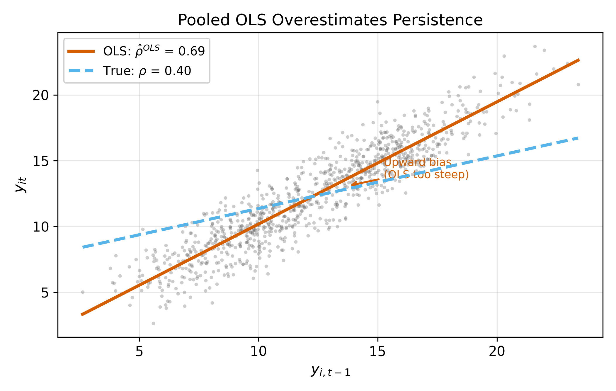
Figure 12.3 shows this bias in action. The OLS line is steeper than the true relationship because it picks up both genuine persistence (\(\rho\)) and the spurious correlation induced by \(\alpha_i\).
12.3 Why Fixed Effects Also Fails: Nickell Bias
The natural response is to use fixed effects, which eliminates \(\alpha_i\) by demeaning. But here the within transformation creates a new problem.
Recall the demeaned model. Define \(\ddot{y}_{it} = y_{it} - \bar{y}_i\) and \(\ddot{\varepsilon}_{it} = \varepsilon_{it} - \bar{\varepsilon}_i\). After demeaning Equation 12.1:
\[ \ddot{y}_{it} = \rho \, \ddot{y}_{i,t-1} + \beta \, \ddot{x}_{it} + \ddot{\varepsilon}_{it} \]
The trouble is that \(\ddot{y}_{i,t-1}\) and \(\ddot{\varepsilon}_{it}\) are mechanically correlated. To see why, expand both:
- \(\ddot{y}_{i,t-1} = y_{i,t-1} - \bar{y}_i\) contains \(-\bar{\varepsilon}_i = -\frac{1}{T}\sum_{s=1}^{T} \varepsilon_{is}\), which includes \(-\frac{1}{T}\varepsilon_{it}\)
- \(\ddot{\varepsilon}_{it} = \varepsilon_{it} - \bar{\varepsilon}_i\) also contains \(-\bar{\varepsilon}_i\)
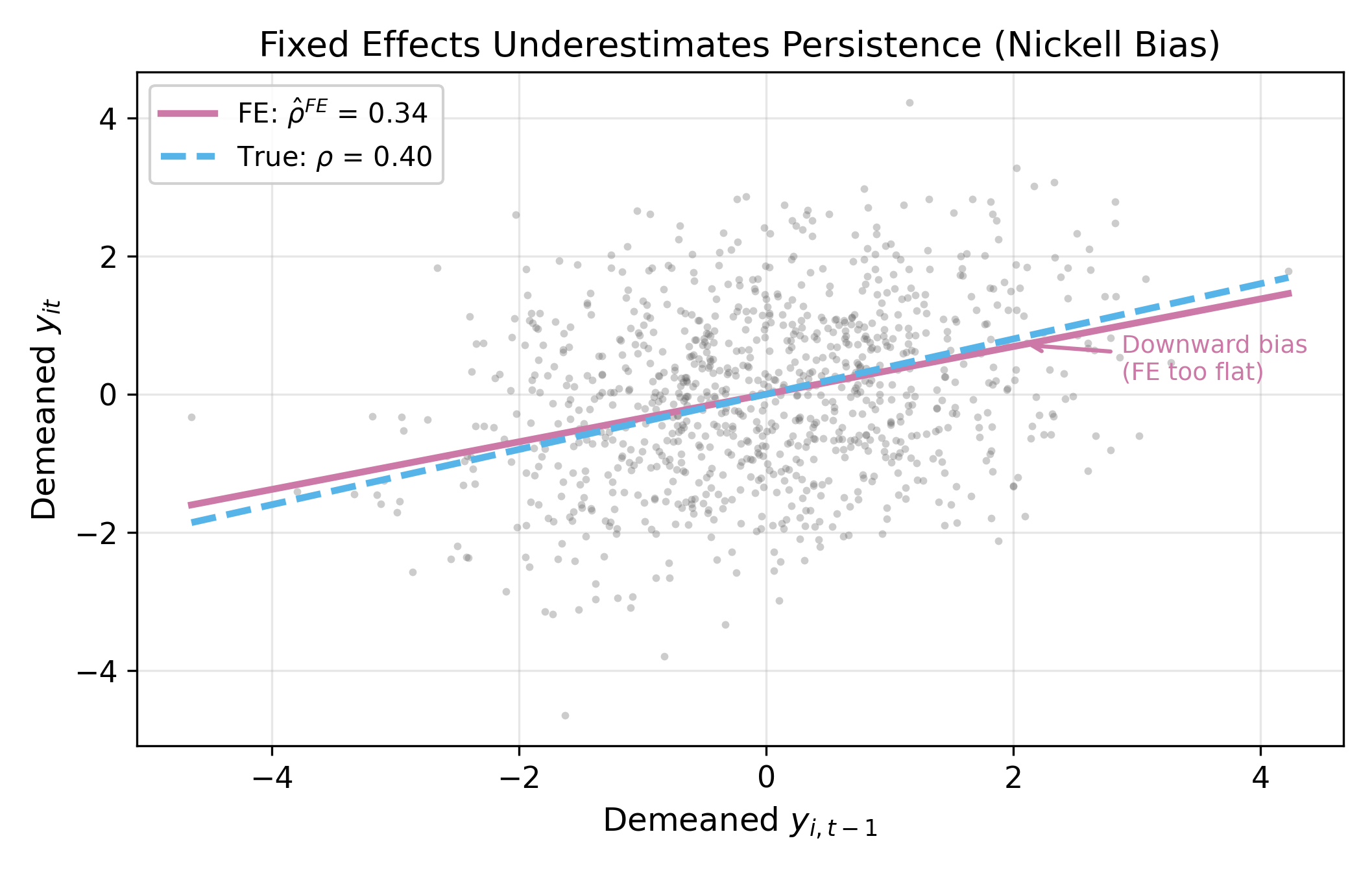
Both the regressor and the error share common terms through \(\bar{\varepsilon}_i\). This creates a negative correlation between \(\ddot{y}_{i,t-1}\) and \(\ddot{\varepsilon}_{it}\), which biases the FE estimator downward.
Nickell (1981) showed the FE bias is \(O(1/T)\), so it vanishes for long panels but is severe when \(T\) is small.
\(\implies\) OLS gives an upper bound for \(\rho\); FE gives a lower bound. The true value lies somewhere in between. If your OLS and FE estimates bracket a narrow range, you can be fairly confident about the true \(\rho\). If they diverge widely, you need a better estimator.
How severe is the bias? It depends on \(T\). Figure 12.5 shows the FE bias as a function of the number of time periods. With \(T = 5\), the bias can be enormous. With \(T = 30\), it is often small enough to ignore.
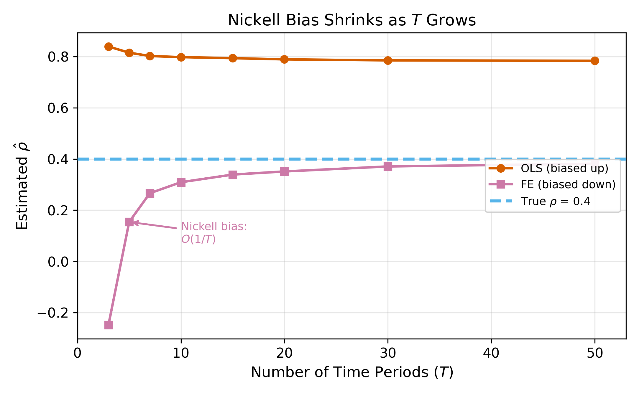
The problematic term is \(-\bar{\varepsilon}_i = -\frac{1}{T}\sum_{s=1}^{T}\varepsilon_{is}\). As \(T\) increases, each individual \(\varepsilon_{it}\) contributes a fraction \(1/T\) to the mean. The mechanical correlation between \(\ddot{y}_{i,t-1}\) and \(\ddot{\varepsilon}_{it}\) is driven by these \(1/T\) terms, so it shrinks toward zero. In the limit \(T \to \infty\), the demeaned regressor and demeaned error are asymptotically uncorrelated, and FE is consistent.
12.4 Arellano-Bond GMM
Arellano and Bond (1991) proposed a two-step solution that avoids both the OLS and Nickell bias problems.
Step 1: First-difference to eliminate \(\alpha_i\).
Instead of demeaning, take first differences of Equation 12.1:
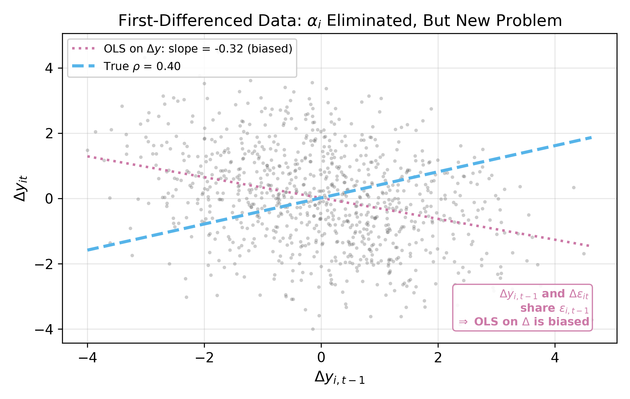
\[ \Delta y_{it} = \rho \, \Delta y_{i,t-1} + \beta \, \Delta x_{it} + \Delta \varepsilon_{it} \tag{12.2}\]
where \(\Delta y_{it} = y_{it} - y_{i,t-1}\). The fixed effect \(\alpha_i\) drops out because it is constant over time: \(\alpha_i - \alpha_i = 0\).
But first-differencing creates its own endogeneity problem. Expand the terms:
- \(\Delta y_{i,t-1} = y_{i,t-1} - y_{i,t-2}\) contains \(\varepsilon_{i,t-1}\)
- \(\Delta \varepsilon_{it} = \varepsilon_{it} - \varepsilon_{i,t-1}\) also contains \(\varepsilon_{i,t-1}\)
So \(\Delta y_{i,t-1}\) and \(\Delta \varepsilon_{it}\) share \(\varepsilon_{i,t-1}\), making OLS on Equation 12.2 inconsistent.
First differencing and demeaning both eliminate \(\alpha_i\), but they create different correlation structures in the transformed errors. Anderson and Hsiao (1981) proposed using lagged levels as instruments for the first-differenced equation; Arellano and Bond extended this to a GMM framework that exploits all available moment conditions.
Step 2: Use lagged levels as instruments.
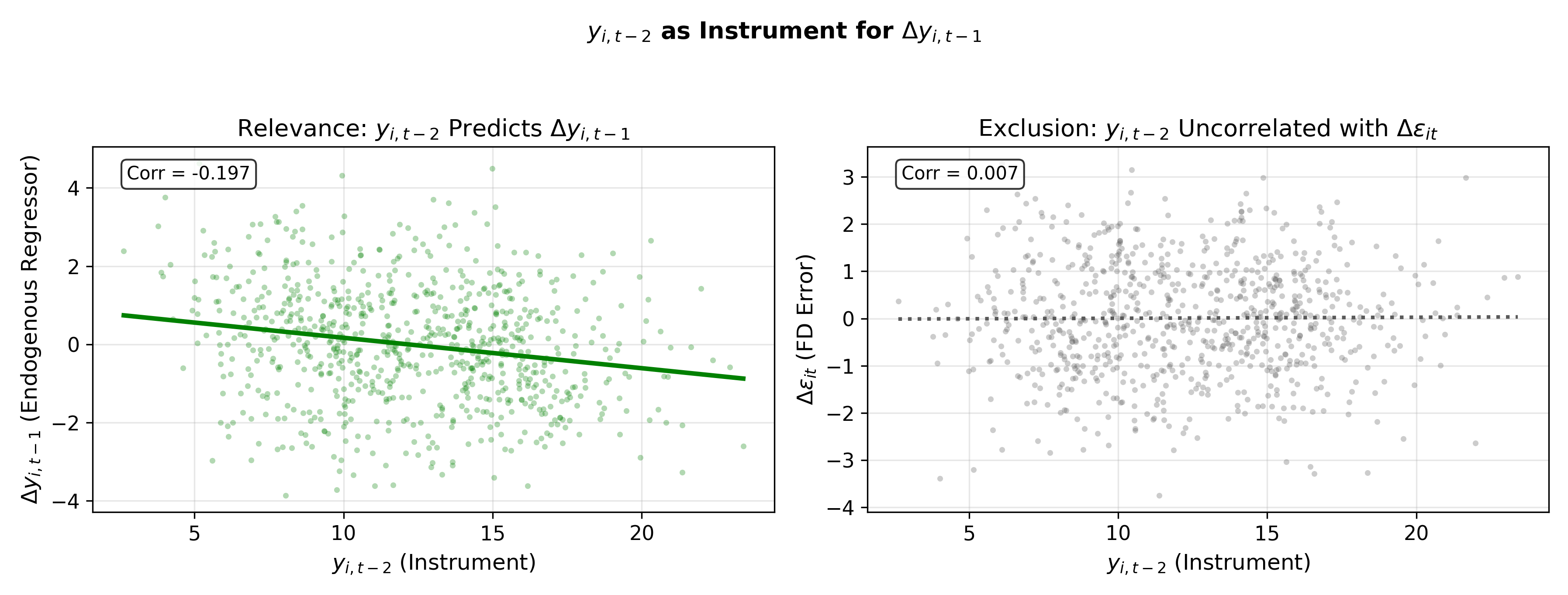
The solution is to instrument \(\Delta y_{i,t-1}\) with \(y_{i,t-2}\). This works because:
- Relevance: \(y_{i,t-2}\) is correlated with \(\Delta y_{i,t-1} = y_{i,t-1} - y_{i,t-2}\) (it appears directly in the expression)
- Exogeneity: \(y_{i,t-2}\) is uncorrelated with \(\Delta \varepsilon_{it} = \varepsilon_{it} - \varepsilon_{i,t-1}\), provided \(\varepsilon_{it}\) is serially uncorrelated
The formal moment condition is:
\[ E[y_{i,s} \cdot \Delta \varepsilon_{it}] = 0 \quad \text{for all } s \leq t-2 \tag{12.3}\]
This means not just \(y_{i,t-2}\) but also \(y_{i,t-3}, y_{i,t-4}, \ldots\) are all valid instruments. Arellano-Bond GMM exploits this full set of moment conditions, building a growing instrument matrix as \(t\) increases.
The moment condition in Equation 12.3 requires \(E[y_{i,s} \cdot \Delta\varepsilon_{it}] = 0\) for \(s \leq t-2\). Since \(\Delta\varepsilon_{it} = \varepsilon_{it} - \varepsilon_{i,t-1}\), any \(y_{i,s}\) with \(s \leq t-2\) was determined before either \(\varepsilon_{it}\) or \(\varepsilon_{i,t-1}\) were realized (assuming no serial correlation in \(\varepsilon\)). So \(y_{i,t-3}\), \(y_{i,t-4}\), and all earlier lags are valid instruments. Using more instruments improves efficiency, though at the cost of potential finite-sample bias from instrument proliferation.
12.5 Results and Diagnostics
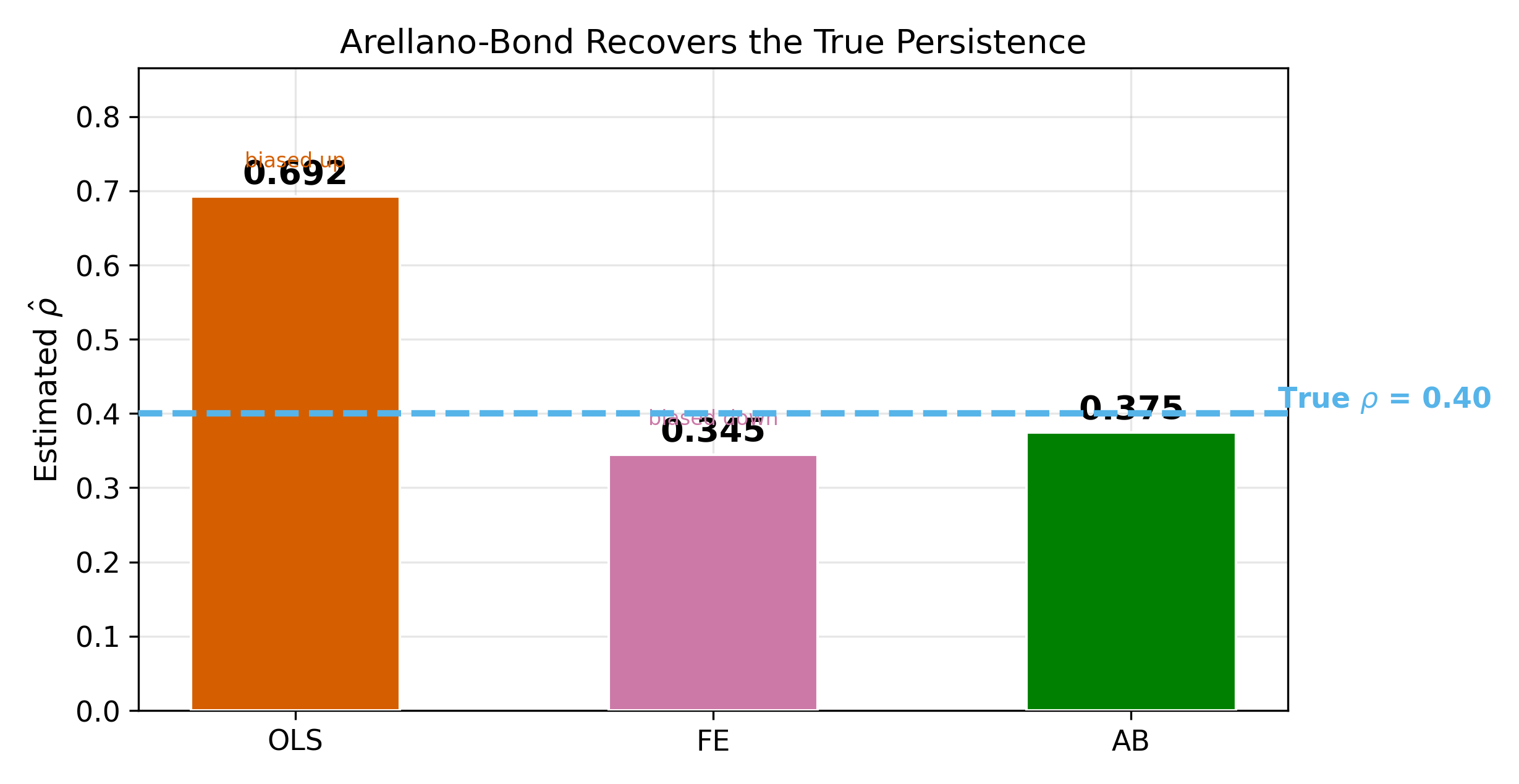
Figure 18.5 summarizes the estimation results across methods. The true \(\rho\) lies between the OLS estimate (biased up) and the FE estimate (biased down), with Arellano-Bond centered on the true value.
Two diagnostic tests are essential when using Arellano-Bond:
12.5.1 AR(2) Test
The moment conditions in Equation 12.3 assume no serial correlation in the level errors \(\varepsilon_{it}\). First-differencing mechanically introduces AR(1) in \(\Delta\varepsilon_{it}\) (since \(\Delta\varepsilon_{it}\) and \(\Delta\varepsilon_{i,t-1}\) share \(\varepsilon_{i,t-1}\)), so AR(1) in the differenced residuals is expected and uninformative. But AR(2) in the differenced residuals would indicate AR(1) in the level errors, which invalidates the instruments.
\(\implies\) Test for second-order autocorrelation in the first-differenced residuals. Failure to reject is what you want.
12.5.2 Sargan/Hansen Test
With more instruments than parameters, you can test whether the overidentifying restrictions hold. The Sargan test (under homoskedasticity) or Hansen J-test (robust to heteroskedasticity) tests the null that all instruments are jointly valid.
\(\implies\) Failure to reject means the instruments appear valid. Rejection suggests at least one moment condition is violated.
A common pitfall: when the number of instruments is large relative to \(N\), the Sargan/Hansen test loses power and rarely rejects, even when instruments are invalid. Always check whether the instrument count is reasonable.
12.5.3 When Arellano-Bond Struggles
AB can perform poorly in several situations:
- Small \(T\): Fewer time periods means fewer available instruments, reducing efficiency
- Weak instruments: When \(\rho\) is close to 1 (near unit root), lagged levels are weakly correlated with first differences, and the instruments become uninformative
- Instrument proliferation: Using the full set of available lags creates a large instrument matrix that can overfit in finite samples, biasing results toward the endogenous estimators
12.6 System GMM: Blundell-Bond
Blundell and Bond (1998) proposed a refinement that addresses the weak-instrument problem. The idea is to use two sets of equations simultaneously:
- Differenced equations (same as AB): instruments are lagged levels (\(y_{i,t-2}, y_{i,t-3}, \ldots\))
- Level equations (new): instruments are lagged differences (\(\Delta y_{i,t-1}, \Delta y_{i,t-2}, \ldots\))
The additional moment condition for the level equations is:
\[ E[\Delta y_{i,s} \cdot (\alpha_i + \varepsilon_{it})] = 0 \quad \text{for } s \leq t-1 \]
This requires a stationarity condition on the initial observations: the correlation between \(\alpha_i\) and \(y_{i1}\) must be constant across individuals. Under this assumption, lagged differences are valid instruments for the level equation because they are correlated with \(y_{i,t-1}\) but uncorrelated with \(\alpha_i + \varepsilon_{it}\).
System GMM combines both sets of moment conditions, yielding a more efficient estimator. It is especially valuable when \(\rho\) is large (near unit root), precisely where standard AB suffers from weak instruments.
Rule of thumb: the number of instruments should not exceed the number of groups (\(N\)). When it does, the Hansen test is unreliable and the GMM estimates may be biased toward the uninstrumented estimators.
The trade-off is clear: more instruments bring more efficiency but also more risk of overfitting. Researchers should report results with and without collapsing the instrument matrix, and verify that diagnostic tests remain well-behaved.
12.6.1 One-Step vs. Two-Step GMM
Both AB and system GMM can be estimated in one step or two steps:
- One-step GMM uses a predetermined weight matrix (typically assuming homoskedasticity). It is simple and often preferred for inference because its standard errors are more reliable in finite samples.
- Two-step GMM uses the residuals from the first step to construct an optimal weight matrix, then re-estimates. It is asymptotically more efficient but tends to produce downward-biased standard errors in small samples. Windmeijer (2005) proposed a finite-sample correction that is now standard in software.
\(\implies\) Use two-step GMM with Windmeijer-corrected standard errors as the default. Report one-step results as a robustness check.
In finite samples, each instrument adds a moment condition that the GMM estimator tries to satisfy. With many instruments, the estimator can satisfy all conditions simultaneously by overfitting to the sample rather than identifying the true parameter. This is analogous to overfitting in regression: a model with as many parameters as observations fits perfectly but predicts poorly. In GMM, the symptom is that estimates drift toward the biased OLS or FE values, and the Hansen test loses its ability to detect invalid instruments.
12.7 Decision Flowchart
When faced with a panel model that might include a lagged dependent variable, the following decision tree applies:
- Is \(y_{i,t-1}\) a regressor?
- No \(\implies\) standard FE or RE methods apply (see Section 12.1 in Panel Data Models)
- Yes \(\implies\) proceed to step 2
- Is \(T\) large (say, \(T > 30\))?
- Yes \(\implies\) FE is acceptable; Nickell bias is \(O(1/T)\) and likely negligible (see Figure 12.5)
- No \(\implies\) proceed to step 3
- Is \(\rho\) close to 1 (near unit root)?
- No \(\implies\) Arellano-Bond (difference GMM) should work well
- Yes \(\implies\) use system GMM (Blundell-Bond), since lagged levels are weak instruments for differenced equations
In all GMM cases, report the AR(2) test and Sargan/Hansen test. If either diagnostic fails, reconsider the model specification.
\(T = 20\) is in a gray area. The Nickell bias is \(O(1/T) \approx 5\%\), which may or may not be tolerable depending on the application. A practical approach: estimate both FE and AB. If the estimates are close, FE is fine and simpler to interpret. If they diverge noticeably, prefer AB. Using the OLS-FE bracketing from Section 12.3 can also help gauge the severity of the bias.
The Hausman-Taylor estimator offers a middle ground between FE and RE when some regressors are correlated with the individual effect but you still want to estimate coefficients on time-invariant variables.