21 Regularization
Ridge, Lasso, and Elastic Net for Prediction
With more features than a dataset can reliably support, OLS overfits, it captures noise as if it were signal, producing excellent in-sample fit but poor out-of-sample predictions. Regularization adds a penalty to the OLS objective that shrinks coefficients toward zero. Ridge regression (\(\ell_2\)) shrinks uniformly, Lasso (\(\ell_1\)) performs automatic variable selection, and Elastic Net blends both. Cross-validation selects the penalty strength \(\lambda\).
This page assumes familiarity with OLS regression and the idea of minimizing a sum of squared residuals. See Omitted Variable Bias for the OLS background.
21.1 The Problem: Too Many Features
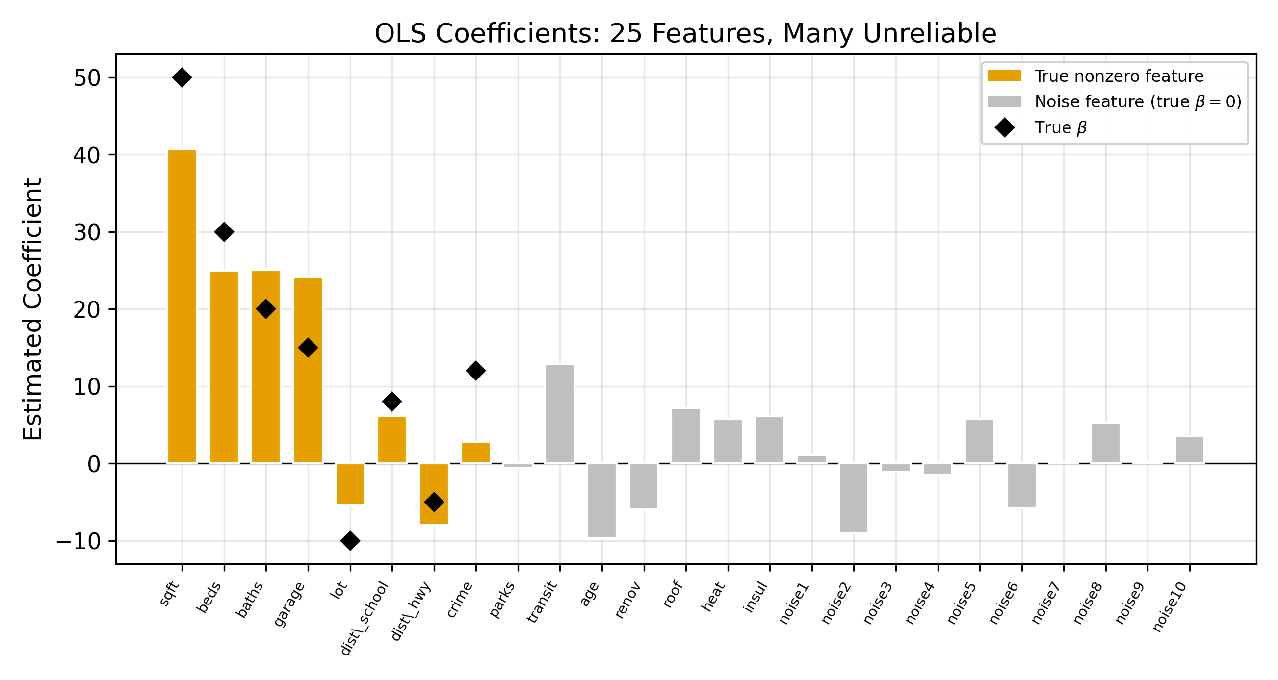
Suppose you have 25 candidate features and 200 observations. OLS will happily estimate all 25 coefficients. It will find the linear combination that fits the training data as closely as possible. The problem is that some of that fit comes from noise.
With 25 features and only 200 observations, OLS has enough degrees of freedom to chase patterns that exist only in this particular sample. The resulting model looks great on the data it was trained on and falls apart on new data. This is overfitting.
\[ \hat{\beta}^{\text{OLS}} = \arg\min_\beta \sum_{i=1}^{n} \bigl(y_i - x_i'\beta\bigr)^2 \tag{21.1}\]
OLS has one goal: minimize the sum of squared residuals. There is no penalty for complexity. A model with 25 large coefficients is treated the same as one with 5 small coefficients, so long as the residuals are smaller.
With \(p > n\) (more features than observations), OLS cannot even be computed. The system is underdetermined, meaning infinitely many coefficient vectors fit the data perfectly. Regularization resolves this by imposing a unique solution.
\(\implies\) When the goal is prediction, minimizing training error alone is not enough. We need a mechanism that discourages the model from becoming too complex.
The core idea of regularization is to add a penalty term to the OLS objective. Instead of minimizing residuals alone, the model minimizes residuals plus a cost for having large coefficients. This forces the optimizer to find coefficient values that fit the data reasonably well and remain small in magnitude. The result is a model that generalizes better to new observations.
21.2 The Bias-Variance Tradeoff
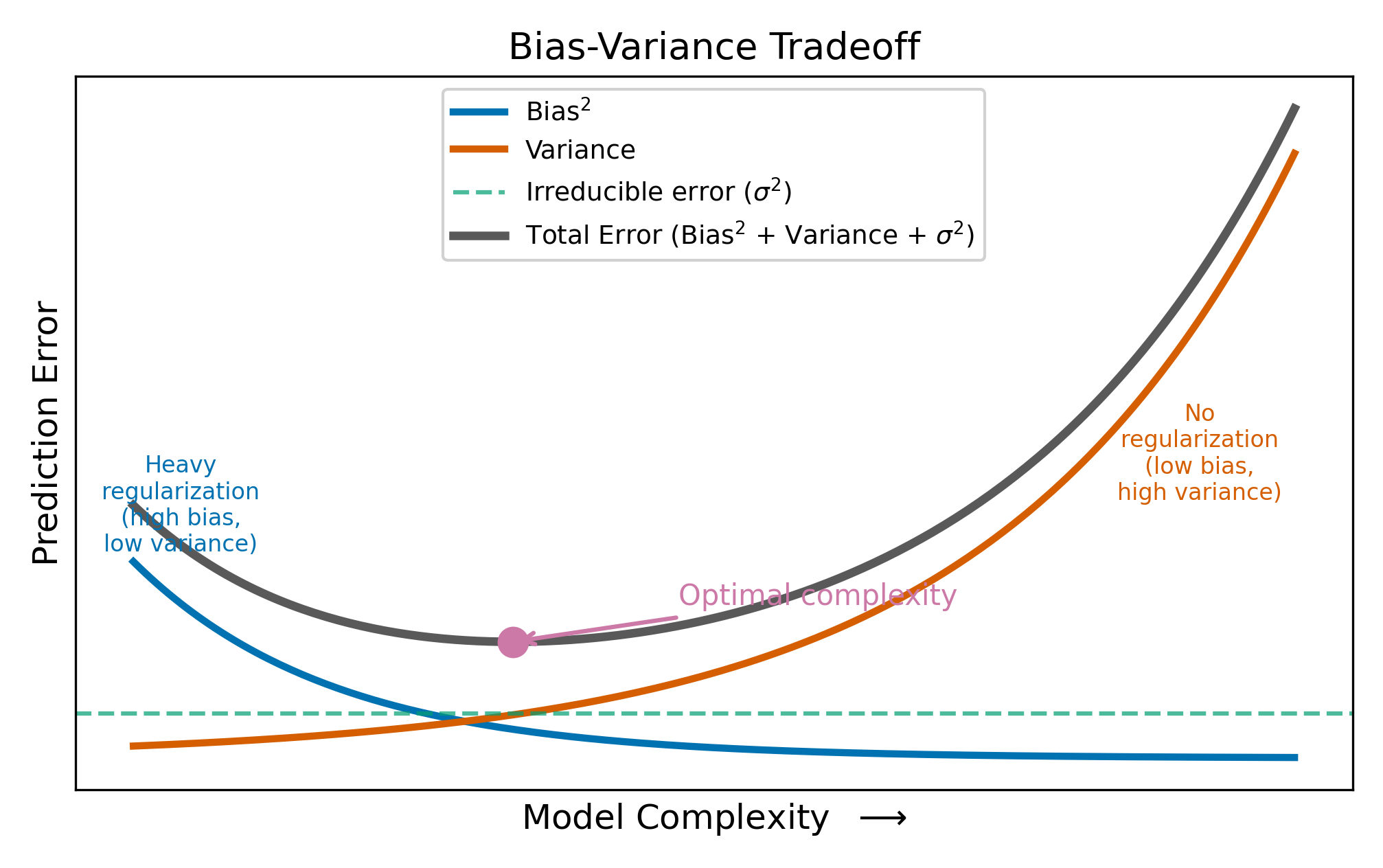
The expected prediction error for a new observation decomposes into three parts:
\[ \text{Expected Prediction Error} = \text{Bias}^2 + \text{Variance} + \sigma^2 \tag{21.2}\]
where \(\sigma^2\) is the irreducible noise in the outcome. You cannot do anything about \(\sigma^2\). The question is how to balance the other two terms.
Bias is the systematic error from using a model that is too simple. If the true relationship involves 5 features but your model only uses 2, the missing features introduce bias.
Variance is the sensitivity of the estimates to the particular sample. If you re-drew the data and re-estimated the model, how much would the coefficients change? OLS on 25 features has high variance because every sample produces a different set of noisy coefficients.
OLS is unbiased: on average, it gets the right answer. But when \(p\) is large relative to \(n\), the variance of the estimates is so high that individual predictions are unreliable. Regularization accepts a small amount of bias in exchange for a large reduction in variance. The net effect on prediction error is often strongly positive.
To make this concrete: suppose the true coefficient on a feature is \(\beta = 2\). OLS might estimate \(\hat{\beta} = 5\) in one sample and \(\hat{\beta} = -1\) in another. The average is correct (unbiased), but any single estimate is far from the truth. A Ridge estimate of \(\hat{\beta} = 1.7\) is slightly biased (it’s too small), but it’s consistently close to the truth across samples. For prediction, consistency beats unbiasedness.
No. With infinite data, there is no estimation variance: OLS would recover the true coefficients exactly. The variance term vanishes, and introducing bias through regularization would only hurt. Regularization is a finite-sample tool. It helps precisely because your dataset is too small to estimate all the parameters reliably.
21.3 Ridge Regression (\(\ell_2\) Penalty)
Ridge regression modifies the OLS objective by adding a penalty proportional to the sum of squared coefficients:
\[ \hat{\beta}^{\text{Ridge}} = \arg\min_\beta \left\{ \sum_{i=1}^{n}(y_i - x_i'\beta)^2 + \lambda \sum_{j=1}^{p} \beta_j^2 \right\} \tag{21.3}\]
The penalty \(\lambda \sum \beta_j^2\) penalizes large coefficients. The tuning parameter \(\lambda \geq 0\) controls the penalty strength:
- When \(\lambda = 0\), the penalty vanishes and Ridge reduces to OLS.
- As \(\lambda \to \infty\), the penalty dominates and all coefficients are driven toward zero.
For a single regressor (with standardized data), the Ridge estimator has a simple closed form:
\[ \hat{\beta}^{\text{Ridge}} = \frac{\sum_{i=1}^{n} x_i y_i}{\sum_{i=1}^{n} x_i^2 + \lambda} \tag{21.4}\]
Compared to the OLS formula \(\hat{\beta}^{\text{OLS}} = \sum x_i y_i / \sum x_i^2\), Ridge adds \(\lambda\) to the denominator. A larger denominator means a smaller coefficient. This is the shrinkage: every coefficient gets pulled toward zero by a factor that depends on \(\lambda\).
Ridge is equivalent to adding \(\lambda\) to the diagonal of the \(X'X\) matrix before inverting, which stabilizes the computation when features are collinear. This is why Ridge is sometimes called “Tikhonov regularization” in applied mathematics.
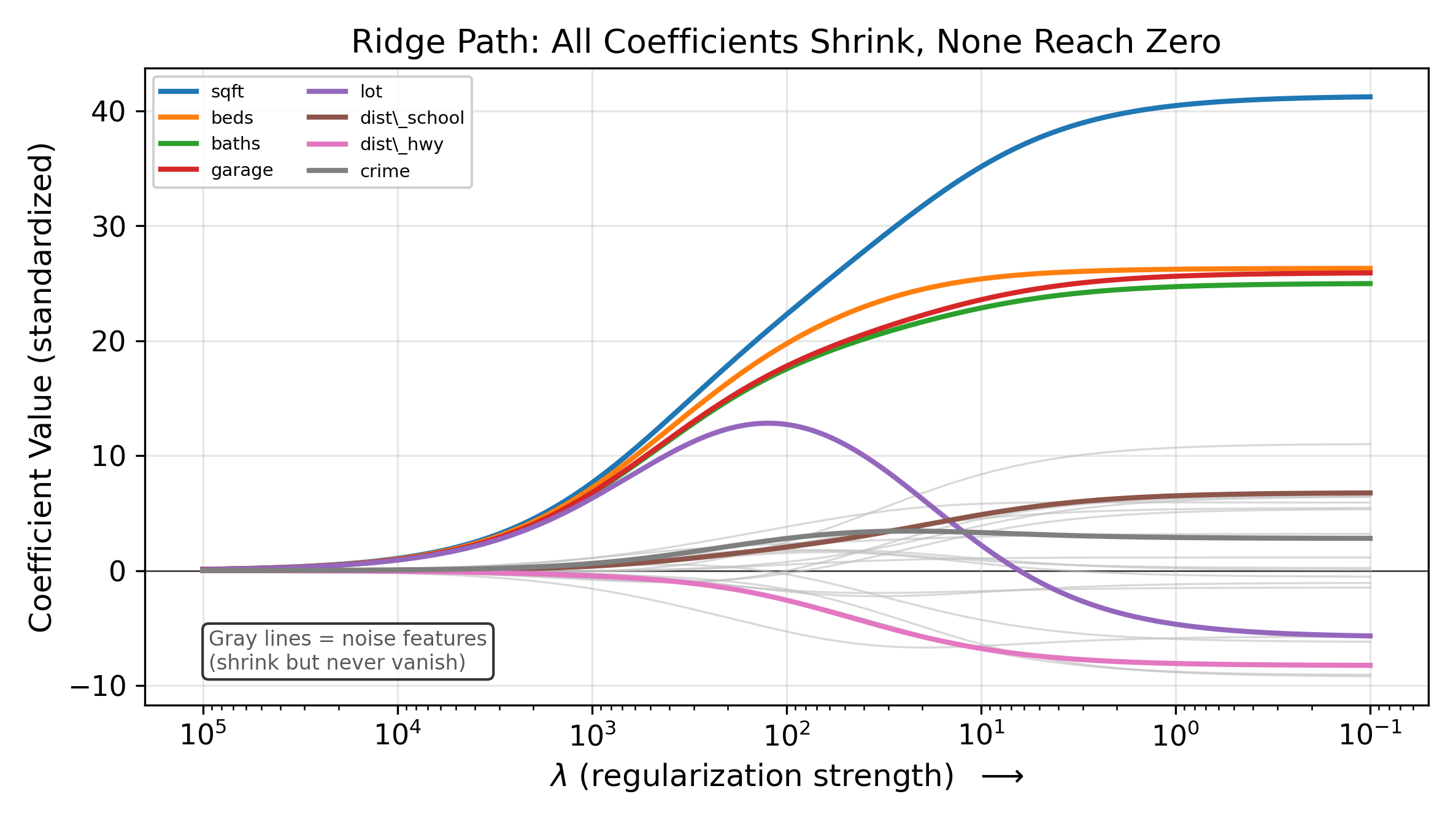
The defining characteristic of Ridge: it shrinks every coefficient toward zero, but it never sets any coefficient exactly to zero. All 25 features remain in the model regardless of how large \(\lambda\) becomes. If your goal includes variable selection, Ridge will not provide it.
21.3.1 The Shrinkage Factor
For the single-regressor case, we can express the Ridge estimate as a fraction of the OLS estimate:
\[ \hat{\beta}^{\text{Ridge}} = \frac{\sum x_i^2}{\sum x_i^2 + \lambda} \cdot \hat{\beta}^{\text{OLS}} \tag{21.5}\]
The ratio \(\sum x_i^2 / (\sum x_i^2 + \lambda)\) is always between 0 and 1. When \(\lambda\) is small relative to \(\sum x_i^2\), the ratio is close to 1 and Ridge barely changes the OLS estimate. When \(\lambda\) is large, the ratio approaches 0 and the coefficient is pulled close to zero. This proportional shrinkage applies to every coefficient in the model.
21.3.2 Why Standardize Before Regularization?
The penalty \(\sum \beta_j^2\) treats all coefficients on the same scale. If one feature is measured in dollars (range: 10,000 to 100,000) and another in years (range: 0 to 40), the dollar feature’s coefficient is mechanically smaller, and the penalty shrinks it less. To ensure the penalty treats all features equally, standardize each feature to have mean zero and unit variance before fitting.
Standardize by subtracting the mean and dividing by the standard deviation: \(\tilde{x}_{ij} = (x_{ij} - \bar{x}_j) / s_j\). After fitting on standardized data, transform the coefficients back to the original scale for interpretation. Note that the intercept is never penalized, since penalizing the intercept would shift all predictions toward zero rather than toward the mean of \(y\).
21.4 Lasso Regression (\(\ell_1\) Penalty)
The Lasso replaces the squared penalty with an absolute value penalty:
\[ \hat{\beta}^{\text{Lasso}} = \arg\min_\beta \left\{ \sum_{i=1}^{n}(y_i - x_i'\beta)^2 + \lambda \sum_{j=1}^{p} |\beta_j| \right\} \tag{21.6}\]
This looks like a minor change, but it has a dramatic consequence: the Lasso sets some coefficients to exactly zero. Unlike Ridge, which keeps all features in the model at reduced magnitude, the Lasso eliminates features entirely. The surviving features form a sparse model that is often easier to interpret.
21.4.1 Why Does the \(\ell_1\) Penalty Produce Zeros?
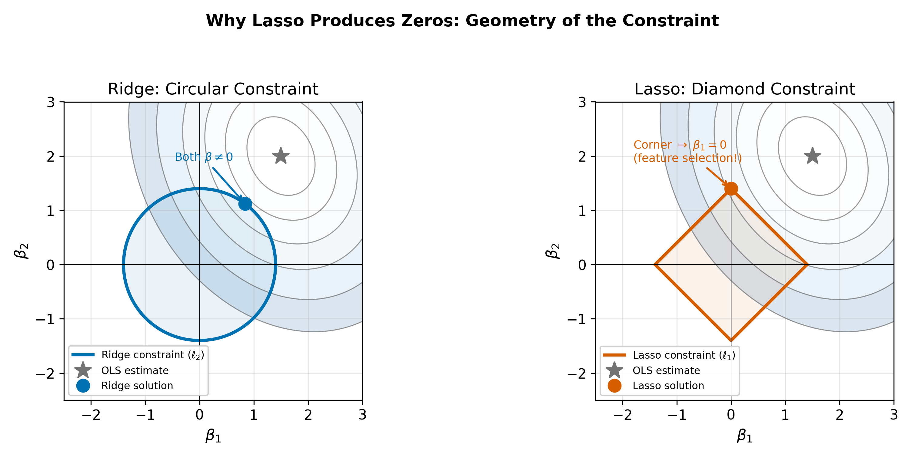
Think of the optimization geometrically. The OLS solution minimizes the residual sum of squares, which traces out elliptical contours in coefficient space. The regularization penalty constrains the coefficients to lie within a budget region:
- Ridge’s \(\sum \beta_j^2 \leq t\) defines a circle (in two dimensions).
- Lasso’s \(\sum |\beta_j| \leq t\) defines a diamond.
The optimal point is where the elliptical contours first touch the constraint region. A circle is smooth, so the point of contact is almost never on an axis. A diamond has corners on the axes, and the ellipses are much more likely to first touch the constraint at a corner, which corresponds to one or more coefficients being exactly zero.
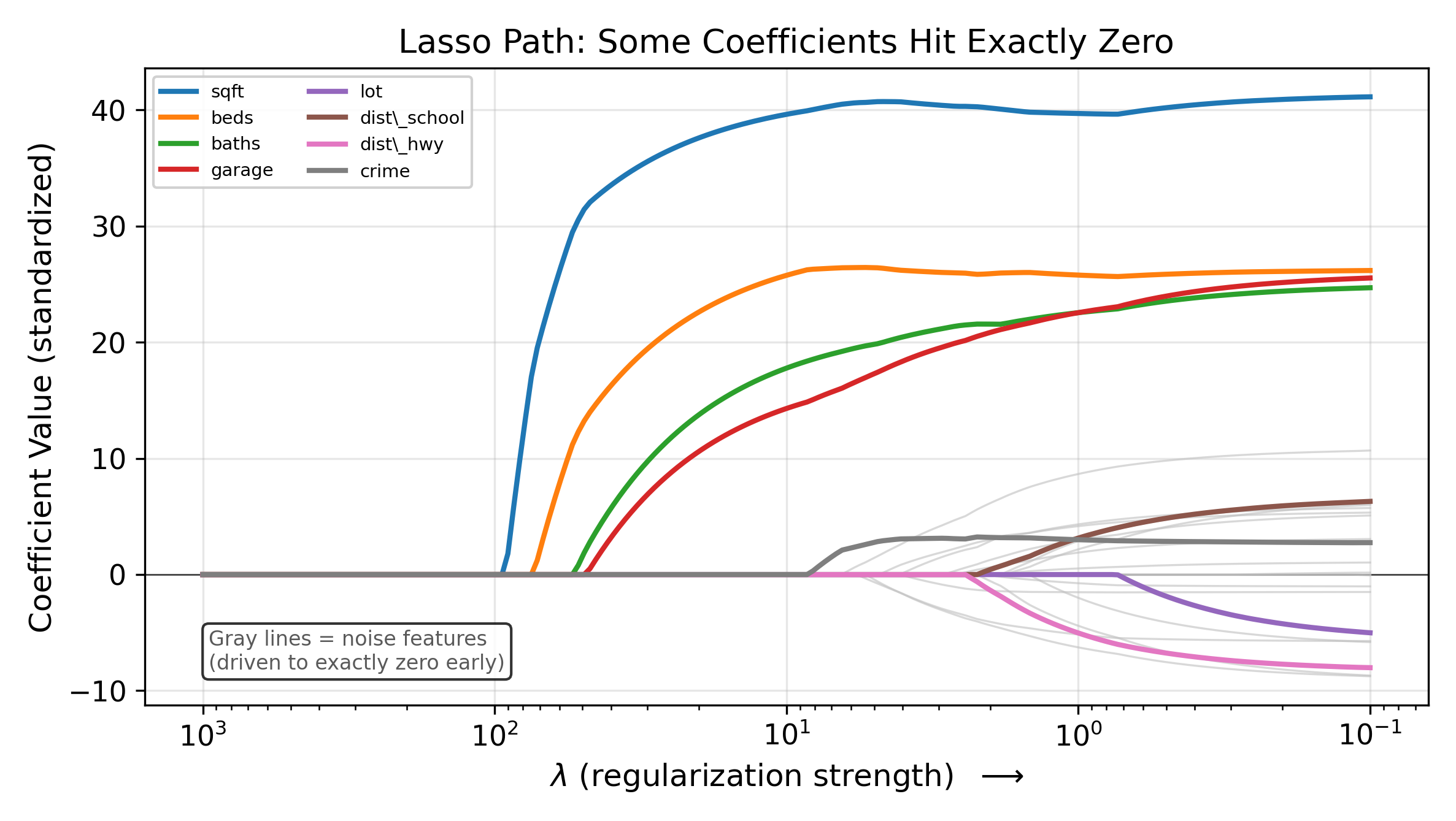
\(\implies\) The Lasso performs automatic variable selection. As \(\lambda\) increases, features drop out of the model one by one. The features that survive at large \(\lambda\) are the ones most strongly associated with the outcome.
21.4.2 A Limitation: The \(n\) Barrier
The Lasso can select at most \(n\) features (where \(n\) is the number of observations). In the \(p > n\) setting, this means many potentially relevant features are excluded even if they carry signal. This is one motivation for the Elastic Net, which does not face this constraint.
The corners of the diamond lie exactly on the coordinate axes, where one or more coefficients equal zero. Elliptical contours approaching a smooth, curved boundary (the circle) will generically make tangential contact at a point where both coordinates are nonzero. But a diamond has flat edges that meet at sharp corners. The ellipse is more likely to first touch the diamond at one of these corners than along a flat edge, because the corner juts out toward the approaching contour. At a corner, at least one coordinate is zero. This geometric argument generalizes to higher dimensions, where the \(\ell_1\) ball has even more corners relative to its faces.
21.5 Elastic Net
The Elastic Net combines both penalties:
\[ \hat{\beta}^{\text{EN}} = \arg\min_\beta \left\{ \sum_{i=1}^{n}(y_i - x_i'\beta)^2 + \lambda\left[\alpha \sum_{j=1}^{p} |\beta_j| + \frac{1-\alpha}{2} \sum_{j=1}^{p} \beta_j^2 \right] \right\} \tag{21.7}\]
The mixing parameter \(\alpha \in [0, 1]\) controls the blend:
- \(\alpha = 1\): pure Lasso (only \(\ell_1\)).
- \(\alpha = 0\): pure Ridge (only \(\ell_2\)).
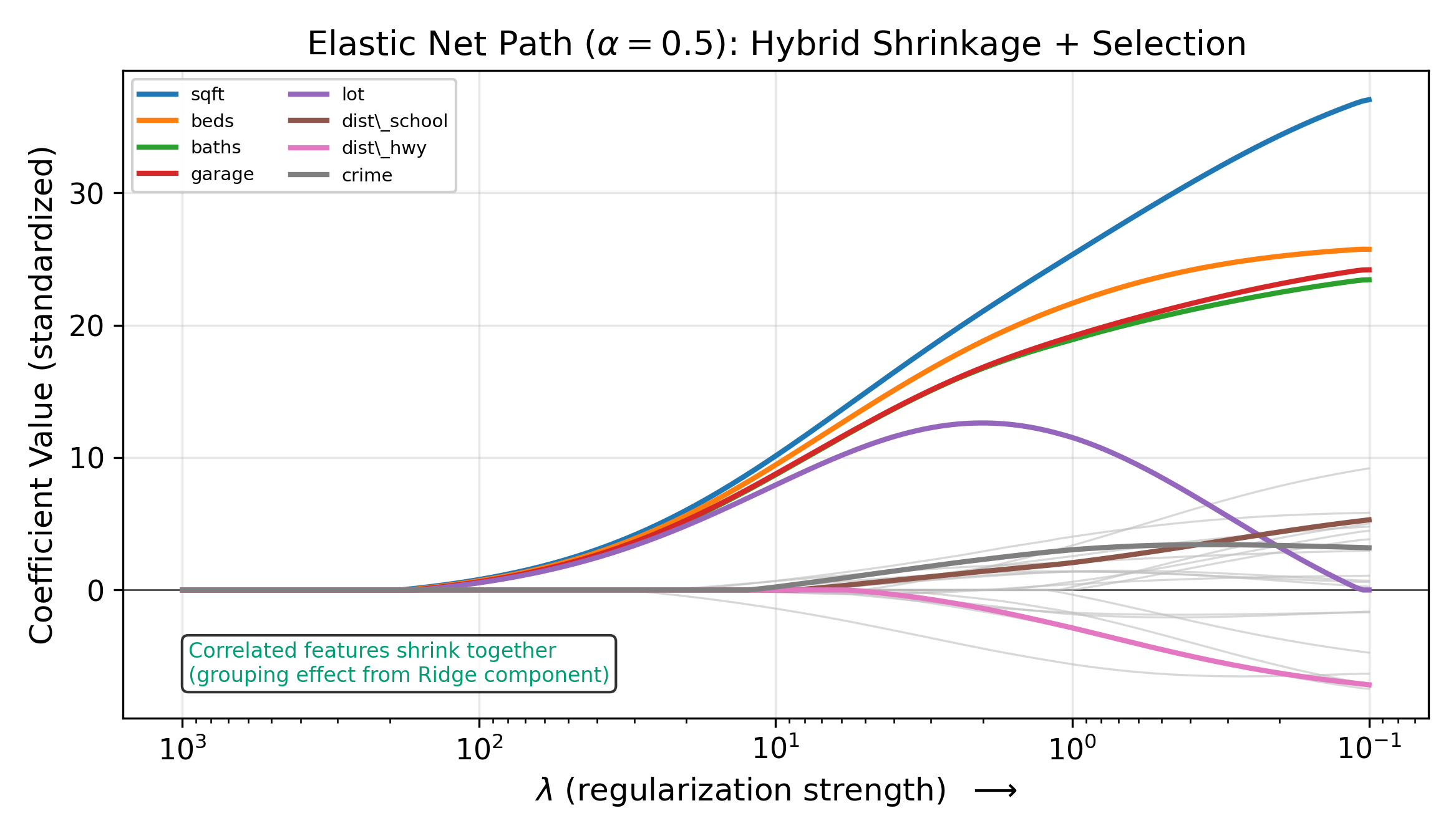
- \(0 < \alpha < 1\): a hybrid that performs variable selection (from the \(\ell_1\) part) while handling correlated features gracefully (from the \(\ell_2\) part).
21.5.1 When Does the Elastic Net Improve on Lasso?
The Lasso has a limitation with correlated features. If two features are highly correlated and both are predictive, the Lasso tends to pick one and zero out the other. Which one it picks can depend on minor sample fluctuations. This instability is problematic when you want a stable set of selected features.
The Elastic Net’s Ridge component encourages correlated features to have similar coefficients rather than forcing a winner-take-all selection. The result is grouped selection: correlated features enter or leave the model together.
The grouped selection property is especially useful in genomics, where genes in the same pathway are often correlated. The Elastic Net selects the pathway rather than a single gene.
In practice, you choose \(\alpha\) by cross-validation alongside \(\lambda\). Common starting points are \(\alpha \in \{0.25, 0.5, 0.75\}\). If your features are mostly uncorrelated, the Elastic Net behaves like the Lasso. If your features have strong group structure, the Ridge component provides stability.
21.5.2 The Elastic Net Constraint Region
Geometrically, the Elastic Net’s constraint region is a blend of the circle and the diamond. At \(\alpha = 0.5\), the boundary is a rounded diamond: it has corners (enabling sparsity) but is less angular than the pure Lasso diamond. As \(\alpha\) increases toward 1, the corners sharpen and the region approaches the Lasso diamond. As \(\alpha\) decreases toward 0, the corners round and the region approaches the Ridge circle.
21.6 Choosing \(\lambda\): Cross-Validation
All three methods require choosing \(\lambda\). Too small, and the penalty has no effect (overfitting). Too large, and the model is over-penalized (underfitting). Cross-validation provides a data-driven answer.
21.6.1 The \(k\)-Fold Procedure
- Randomly split the data into \(k\) folds (typically \(k = 5\) or \(k = 10\)).
- For each candidate value of \(\lambda\):
- Hold out fold \(j\) as test data. Train the model on the remaining \(k - 1\) folds.
- Compute prediction error on the held-out fold \(j\).
- Repeat for \(j = 1, 2, \ldots, k\).
- Average the \(k\) prediction errors to get the CV error for this \(\lambda\).
- Plot CV error against \(\lambda\). Choose the \(\lambda\) that minimizes the CV error.
This is the most common method for tuning \(\lambda\) in practice. By evaluating prediction performance on data that were not used for training, CV provides an honest estimate of out-of-sample error.
The choice of \(k\) involves a tradeoff. Larger \(k\) (e.g., \(k = n\), called leave-one-out CV) uses nearly all the data for training in each fold, reducing bias in the error estimate but increasing computation and variance. Smaller \(k\) (e.g., \(k = 5\)) is faster and produces a more stable error estimate, at the cost of slightly more bias. In practice, \(k = 10\) is a common default that balances these concerns.
21.6.2 The CV Curve and the One-Standard-Error Rule
The CV error curve is typically U-shaped (on a log scale for \(\lambda\)). Let \(\lambda_{\min}\) denote the value that minimizes CV error. The one-standard-error rule recommends a more parsimonious choice: pick the largest \(\lambda\) whose CV error is within one standard error of the minimum. This is \(\lambda_{1\text{se}}\).
\[ \lambda_{1\text{se}} = \max\{\lambda : \text{CV}(\lambda) \leq \text{CV}(\lambda_{\min}) + \text{SE}(\lambda_{\min})\} \tag{21.8}\]
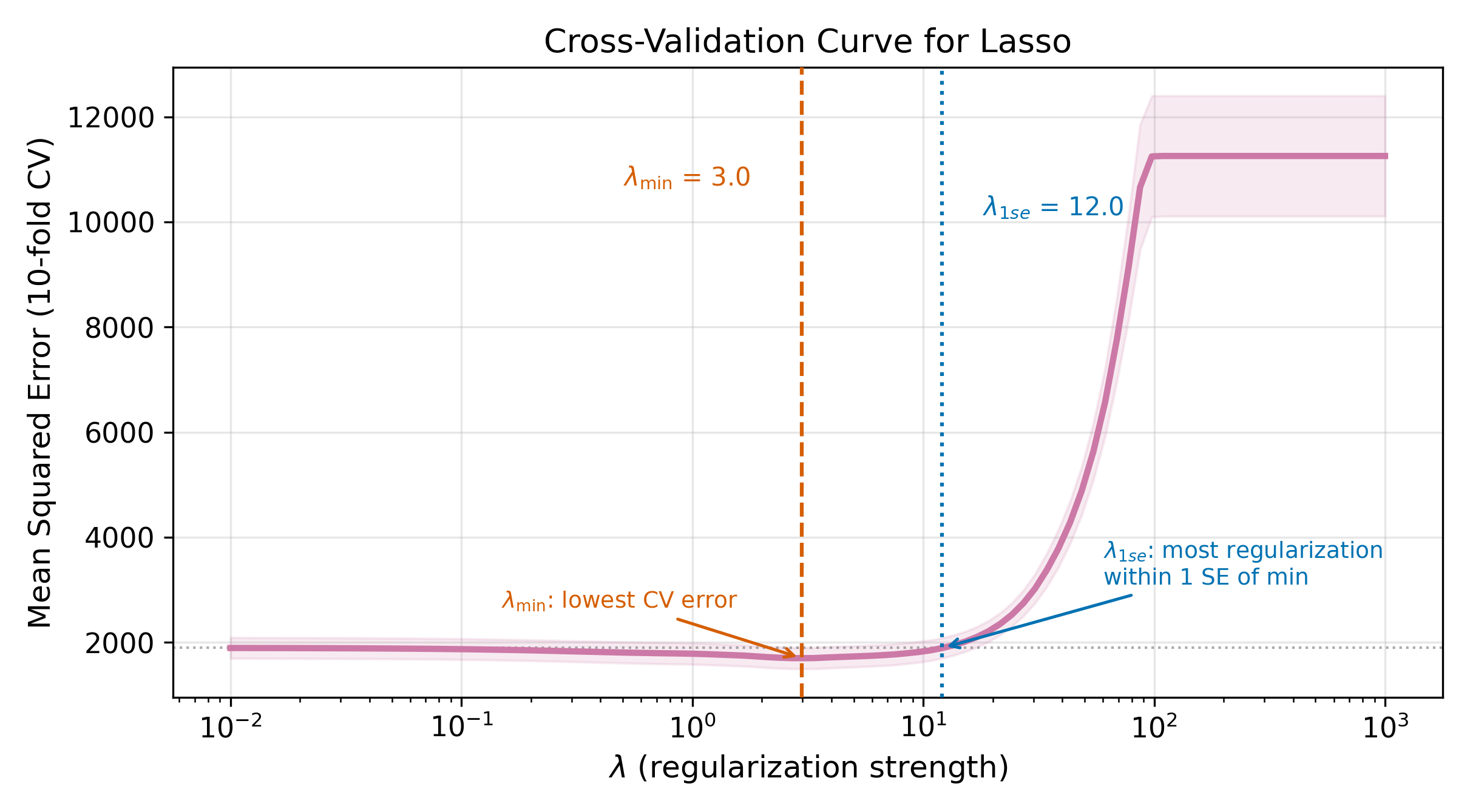
The one-standard-error rule reflects a preference for simplicity. Among all models whose prediction error is statistically indistinguishable from the best, choose the simplest.
\(\lambda_{\min}\) minimizes the estimated CV error, but that estimate itself is noisy. The CV error at \(\lambda_{\min}\) and at nearby values of \(\lambda\) are often statistically indistinguishable. By moving to a slightly larger \(\lambda\), you get a simpler model (fewer nonzero coefficients in Lasso, smaller coefficients in Ridge) with prediction performance within the noise of the optimum. Simpler models are easier to interpret, more stable across samples, and less prone to overfitting. Unless you have a strong reason to squeeze out every last drop of predictive accuracy, \(\lambda_{1\text{se}}\) is the safer choice.
21.7 Comparison
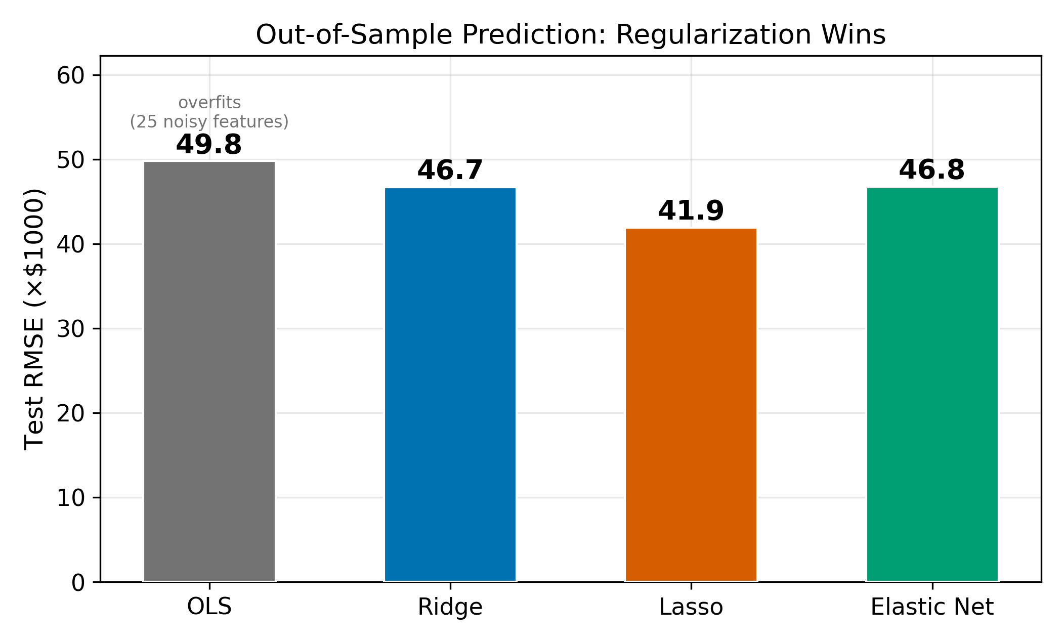
How do these methods perform head-to-head? On a typical dataset with a mix of signal and noise features, OLS overfits, Ridge and Lasso improve substantially, and Elastic Net often matches or slightly beats both.
The relative performance depends on the true data-generating process. When many features have small but nonzero effects, Ridge tends to win because shrinking everything a little is better than zeroing most coefficients out. When only a few features truly matter, Lasso wins because it correctly identifies and retains the sparse signal. Elastic Net is a hedge: it performs well in both scenarios without needing to know the truth in advance.
| Feature | Ridge | Lasso | Elastic Net |
|---|---|---|---|
| Penalty | \(\lambda \sum \beta_j^2\) | \(\lambda \sum |\beta_j|\) | \(\lambda[\alpha\sum|\beta_j| + (1-\alpha)/2 \sum \beta_j^2]\) |
| Variable selection | No | Yes | Yes |
| Handles correlated features | Stable (shrinks together) | Unstable (picks one) | Stable (grouped selection) |
| Number of selected features | Always \(p\) | At most \(n\) | Up to \(p\) |
| Tuning parameters | \(\lambda\) | \(\lambda\) | \(\lambda\) and \(\alpha\) |
| Closed-form solution | Yes | No | No |
| When to use | Many small effects, collinearity | Sparse signal, want interpretability | Correlated features, groups of predictors |
21.8 Regularization Is Not Causal Inference
Everything in this chapter optimizes prediction: minimizing out-of-sample error. The coefficients from Ridge, Lasso, and Elastic Net are biased by design. That bias is the whole point; it reduces variance and improves prediction. But biased coefficients cannot be interpreted as causal effects.
Consider what the Lasso does. It zeros out coefficients for features that do not improve prediction conditional on other features. But a variable can be causal without being a strong predictor (if its effect is small), and a strong predictor can be non-causal (if it is merely correlated with the outcome through a confounder). The Lasso selects for predictive power, not causal relevance.
For causal questions, use the tools from earlier chapters:
- Instrumental variables for endogenous regressors (Chapter 3)
- Fixed effects for unobserved time-invariant confounders (Chapter 15)
- Difference-in-differences for policy evaluation
Post-selection inference (e.g., double Lasso) attempts to bridge the gap by using Lasso to select control variables and then running unpenalized regression on the selected set. This approach has theoretical guarantees under specific conditions, but it is beyond the scope of this course.
\(\implies\) Regularization answers “what predicts \(y\)?” not “what causes \(y\)?” Treat these methods as prediction tools, and reach for causal inference methods when the research question demands it.
This distinction is not just philosophical. In a wage regression, Lasso might drop education and keep occupation, because occupation is a stronger predictor conditional on other variables. But education causes wages through occupation, so dropping it does not mean it is unimportant. The Lasso is optimizing a prediction objective, not tracing causal pathways.
Return to the chapter hub for the full course map. For connections between prediction and causal inference, revisit Instrumental Variables and Panel Data, which address endogeneity rather than prediction accuracy.