10 Random Effects
Modeling Group Heterogeneity as a Random Draw
Fixed effects fix the omitted-variable problem at a cost: one free parameter per group, and zero information on variables that don’t vary within a group. Random effects trades one assumption (group effects uncorrelated with regressors) for two big benefits: dramatically fewer parameters, and the ability to estimate the coefficients of group-level variables. This chapter develops the RE assumption, the error-components model, the intraclass correlation, the GLS partial-demeaning transformation that nests pooled OLS and FE as limiting cases, and the Hausman test for choosing between RE and FE.
10.1 The Setup
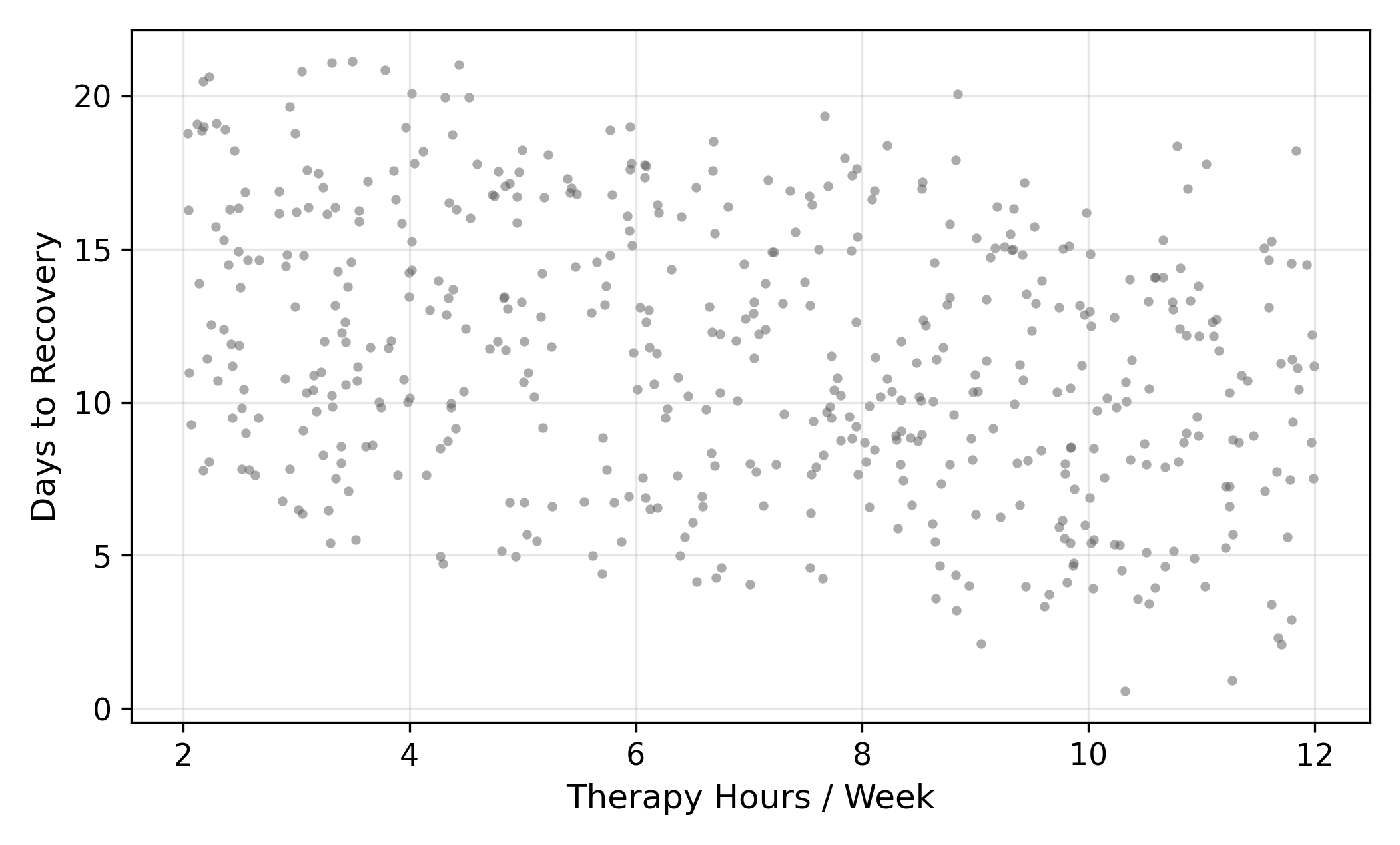
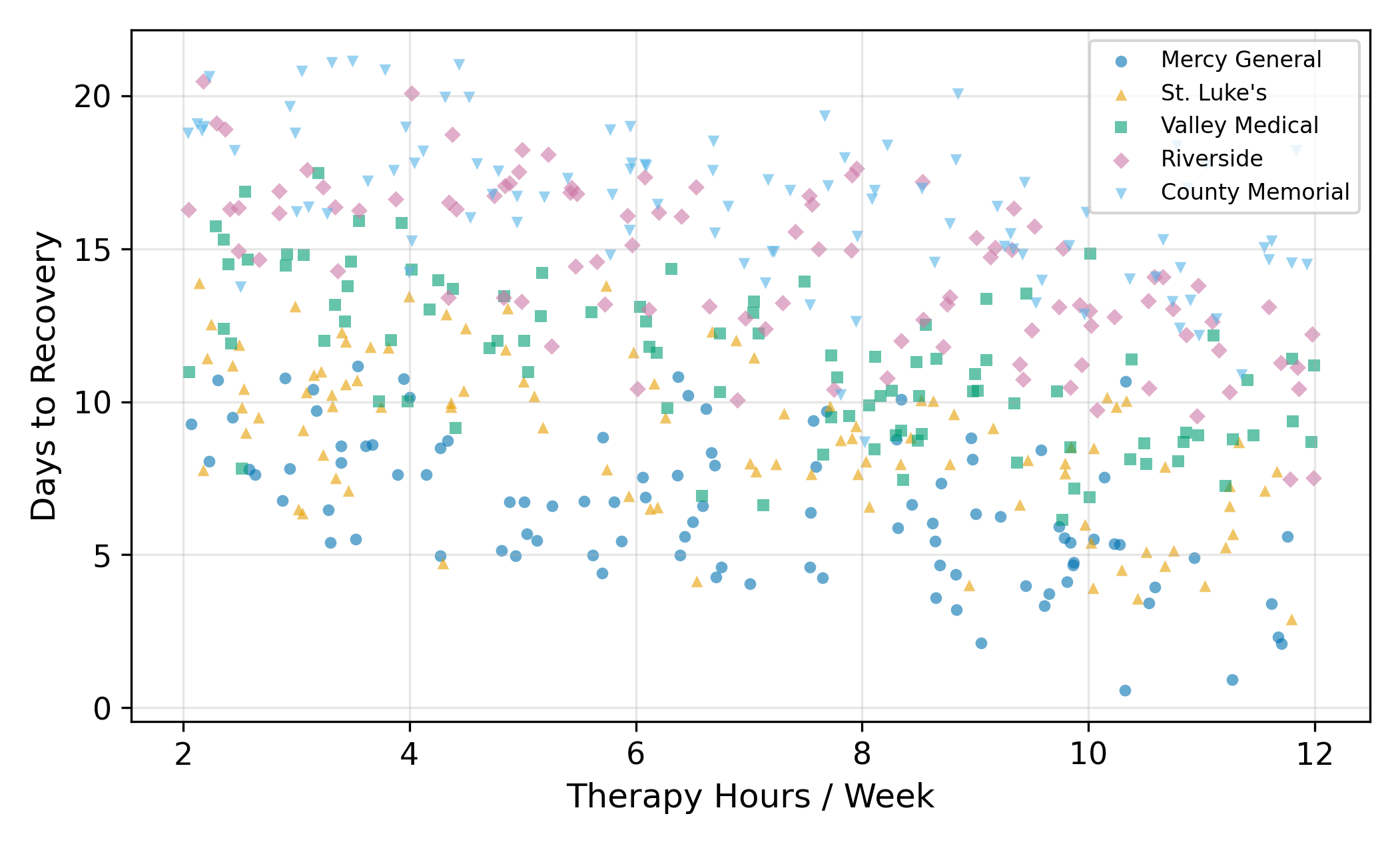
A researcher is studying recovery times after a common surgery. The outcome is days to recovery and the main regressor is hours of physical therapy per week. The data comes from five hospitals: Mercy General, St. Luke’s, Valley Medical, Riverside, and County Memorial.
Each hospital has a different baseline recovery time. Mercy General has newer equipment and faster post-op protocols; County Memorial is a community hospital with longer turnaround. So patients at Mercy recover faster on average than patients at County, holding therapy hours constant. The effect of therapy itself, though, is the same everywhere: more therapy means fewer recovery days.
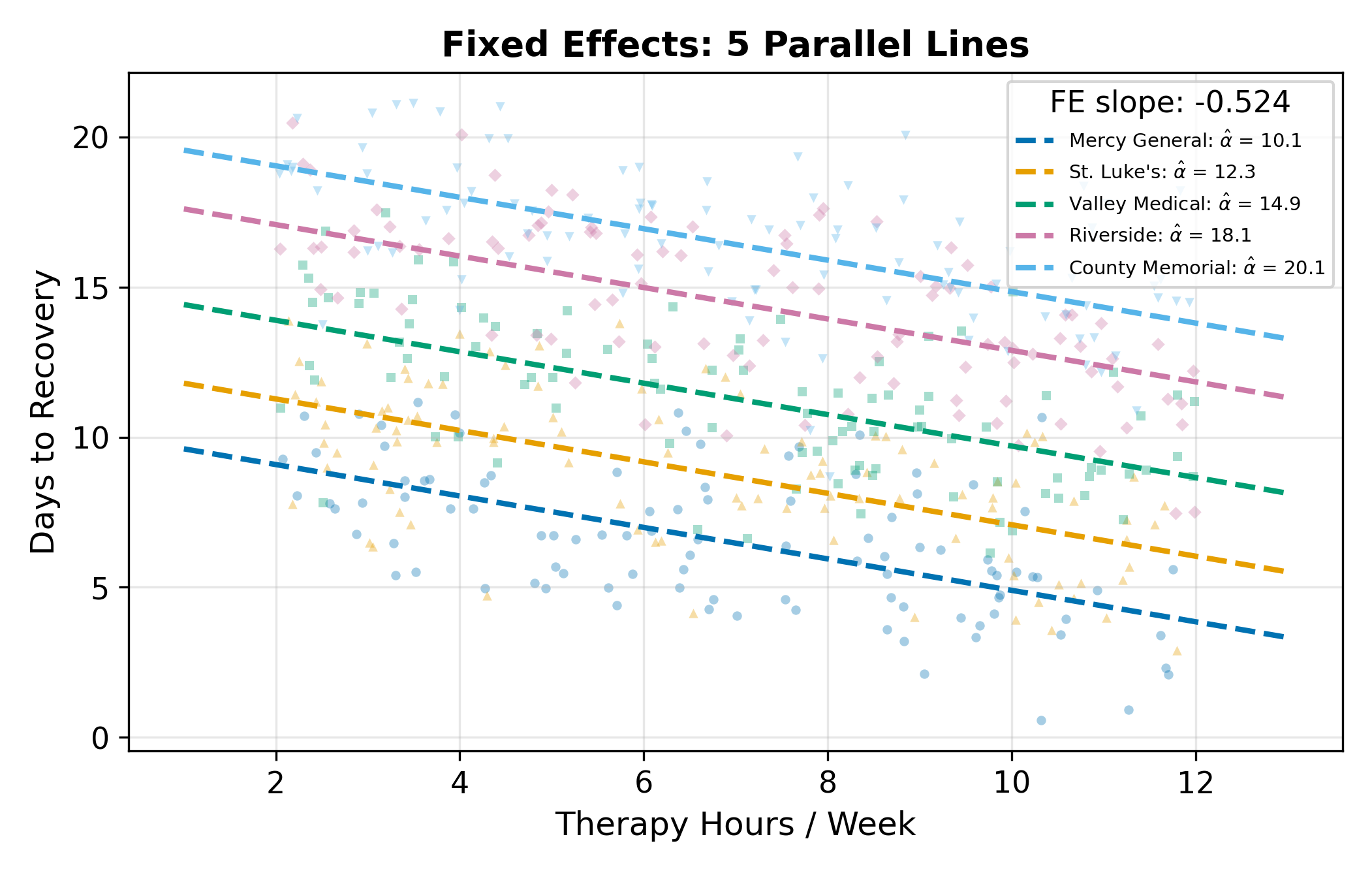
You already know how to handle this with fixed effects. Estimate one intercept per hospital, and the within-hospital slope on therapy gives you the causal effect. FE works, and it works without needing to worry about whether hospital quality and therapy hours are correlated.
So why do we need a new estimator?
10.2 The Cost of Fixed Effects
FE has two real costs, and they bite hard in modern applied work.
Cost 1: a parameter per group. With 5 hospitals, that’s 5 intercepts to estimate. Manageable. With 50 hospitals, 50 intercepts, degrees of freedom start to matter. With 500 (every hospital in a state), 5,000 (every hospital in the country), or 50,000 (every clinic), you are estimating an enormous number of nuisance parameters and the gain from each additional one is tiny. You also burn degrees of freedom that could have gone toward more precise slope estimates.
Cost 2: time-invariant regressors are invisible. This is the more important cost. The within transformation subtracts each unit’s mean, so any variable that doesn’t change within unit becomes zero after demeaning. If you want to know whether teaching hospitals (a permanent attribute of each hospital) recover patients faster, FE can’t tell you. The teaching-status variable gets absorbed into the fixed effect along with everything else.
Lots of questions have this shape. Are rural counties different from urban ones? Do publicly-traded firms invest differently than private ones? Do parliamentary democracies grow faster than presidential ones? Each of those involves a unit-level attribute that doesn’t change over the panel. FE makes them invisible.
The trade-off is structural. FE buys robustness to any unit-level unobserved heterogeneity, and you pay for that with the inability to ask about observed unit-level variables.
Random effects is the deal you can cut to get some of that back.
10.3 The Random Effects Idea
Start from the FE specification, where \(\alpha_j\) is hospital \(j\)’s baseline:
\[ y_{ij} = \alpha_j + \beta \, x_{ij} + \varepsilon_{ij}. \tag{10.1}\]
In FE, each \(\alpha_j\) is treated as a free parameter, five free numbers in our hospital example, separately estimated. Random effects makes a different modeling choice: it treats each \(\alpha_j\) as a draw from a distribution:
\[ \alpha_j = \bar\alpha + u_j, \qquad u_j \sim (0, \sigma_u^2). \tag{10.2}\]
Three pieces to keep straight:
- \(\bar\alpha\) is the average baseline across all hospitals, a single population-level parameter.
- \(u_j\) is hospital \(j\)’s random deviation from that average. It plays the same role as \(\alpha_j\) did in FE, but instead of being a free parameter, it’s a draw from a distribution with mean zero and variance \(\sigma_u^2\).
- \(\sigma_u^2\) measures how spread out hospital baselines are around their common mean.
The key economy: instead of estimating \(J\) separate \(\alpha_j\)’s, you estimate one mean \(\bar\alpha\) and one variance \(\sigma_u^2\). With \(J = 500\), that’s \(500\) parameters collapsed into \(2\). With \(J = 50{,}000\), into \(2\) still.
The distributional model in Equation 10.2 is sometimes called the error components model because it splits the residual into a hospital-level piece (\(u_j\)) and a patient-level piece (\(e_{ij}\)).
10.3.1 The Critical Assumption
RE comes with a price tag, and it’s the assumption that makes everything work:
\[ \operatorname{Cov}(u_j, x_{ij}) = 0. \tag{10.3}\]
In words: the hospital-level random deviation \(u_j\) is uncorrelated with the regressor of interest \(x_{ij}\). Patients at a “better” hospital (one with \(u_j < 0\), meaning lower expected recovery days) can’t systematically receive more (or less) therapy than patients at a “worse” one. If hospital quality and therapy hours are correlated, because better hospitals push more aggressive protocols, or because sicker patients select into better hospitals, then this assumption is violated and RE gives the wrong answer.
This is a strong assumption. The whole reason FE works without anything analogous is that FE doesn’t make this assumption: by demeaning, it allows arbitrary correlation between \(\alpha_j\) and \(x_{ij}\). RE buys back efficiency and the ability to estimate time-invariant variables by promising that the correlation isn’t there.
We come back to whether this assumption is plausible. For now, accept it as a maintained hypothesis and see what it lets us do.
10.4 The Error Components Model
Substitute Equation 10.2 into Equation 10.1:
\[ y_{ij} = \bar\alpha + \beta\,x_{ij} + \underbrace{u_j + e_{ij}}_{\textstyle v_{ij}}. \tag{10.4}\]
The composite error \(v_{ij} = u_j + e_{ij}\) has two parts. The hospital-level component \(u_j\) is identical for every patient at hospital \(j\), and it varies only across hospitals. The idiosyncratic component \(e_{ij}\) is patient-specific noise. With this setup, the model looks like a standard regression with an intercept \(\bar\alpha\), a slope \(\beta\), and an error term \(v_{ij}\).
The problem is that \(v_{ij}\) is not i.i.d. Two patients at Mercy General share the same \(u_{\text{Mercy}}\). Their composite errors are positively correlated. OLS standard errors assume independence, so they are wrong (specifically, too small) when applied to this model.
10.4.1 Within-Group vs. Between-Group Correlation
Compute the correlation between two composite errors. For two patients \(i \neq k\) at the same hospital \(j\):
\[ \operatorname{Corr}(v_{ij}, v_{kj}) = \frac{\operatorname{Cov}(u_j + e_{ij},\; u_j + e_{kj})}{\sigma_u^2 + \sigma_e^2} = \frac{\sigma_u^2}{\sigma_u^2 + \sigma_e^2}. \tag{10.5}\]
That ratio has a name: the intraclass correlation (or rho), often written \(\rho\). It is the share of the total error variance that is due to hospital-level effects. For two patients at different hospitals (\(j \neq \ell\)), the errors are independent and \(\operatorname{Corr}(v_{ij}, v_{k\ell}) = 0\).
The qualitative picture:
- \(\rho \approx 0\): hospitals are basically interchangeable, almost all error is patient-specific noise. Grouping doesn’t tell you much.
- \(\rho \approx 1\): almost all variation is between hospitals, knowing the hospital tells you nearly everything about expected recovery time.
This positive within-group correlation is exactly why OLS standard errors fail: OLS treats every observation as an independent draw, but patients at the same hospital are not independent draws.
A rough rule (the “design effect” from cluster-sampling theory) is that the effective sample size for the unit-level mean is \(N_j / [1 + (N_j - 1)\rho]\). Here \(50 / [1 + 49(0.8)] = 50 / 40.2 \approx 1.24\). The 50 patients at Mercy contain about as much information as \(1.24\) truly independent observations of Mercy’s average recovery time.
That is a dramatic shrinkage. It’s why high within-cluster correlation makes cluster-robust standard errors so much larger than naive OLS SEs. See Cluster-Robust SEs for the inference side of this story.
10.4.2 Borrowing Strength Across the Ensemble
The other reason RE is interesting (besides the parameter economy) is that the correlation structure lets the estimator borrow strength across hospitals. A single hospital with only 5 patients gives you a very noisy local average. But that hospital is one of many, and the whole ensemble carries information about what to expect. The RE estimator combines a hospital’s own data with the ensemble information in proportions that depend on how much of each is reliable.
When a hospital has many patients, the estimator trusts the hospital’s own data and pulls toward the local average. When a hospital has few patients, the estimator pulls more toward the overall mean. The trade-off is automatic, the GLS weights take care of it.
This is the same idea behind Stein-style shrinkage estimation (Efron and Morris, 1973). It is also why mixed-effects models are everywhere in education research, biostatistics, and any setting with many small groups: they aggregate information across groups without requiring each group to provide all its own evidence.
10.5 Estimation: Partial Demeaning
OLS on Equation 10.4 ignores the correlation in \(v_{ij}\) and produces wrong standard errors. Feasible GLS transforms the data so the transformed errors are i.i.d., then runs OLS on the transformation. For the random-effects model the transformation has a clean form.
Define the parameter
\[ \hat\alpha_j = 1 - \frac{\sigma_e}{\sqrt{N_j \sigma_u^2 + \sigma_e^2}}, \tag{10.6}\]
where \(N_j\) is the number of observations in group \(j\). The RE transformation is partial demeaning:
\[ y_{ij}^* = y_{ij} - \hat\alpha_j\, \bar y_j, \qquad x_{ij}^* = x_{ij} - \hat\alpha_j\, \bar x_j. \tag{10.7}\]
Then run OLS on the starred variables. That’s it. Mechanically, RE is OLS on a transformed data set; the transformation just rescales how much of each group’s mean is subtracted.
The constant \(\hat\alpha_j\) in Equation 10.6 is purely a function of the variance components \(\sigma_u^2\) and \(\sigma_e^2\) (which are estimated from the OLS residuals first) and the group size \(N_j\). It is not the same \(\alpha_j\) as the group-level random effect, it’s the GLS weight.
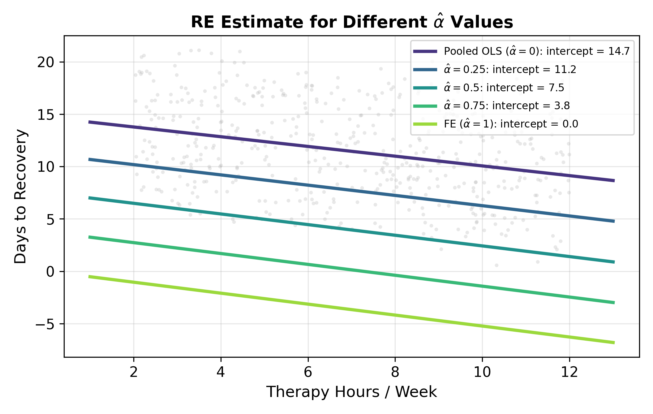
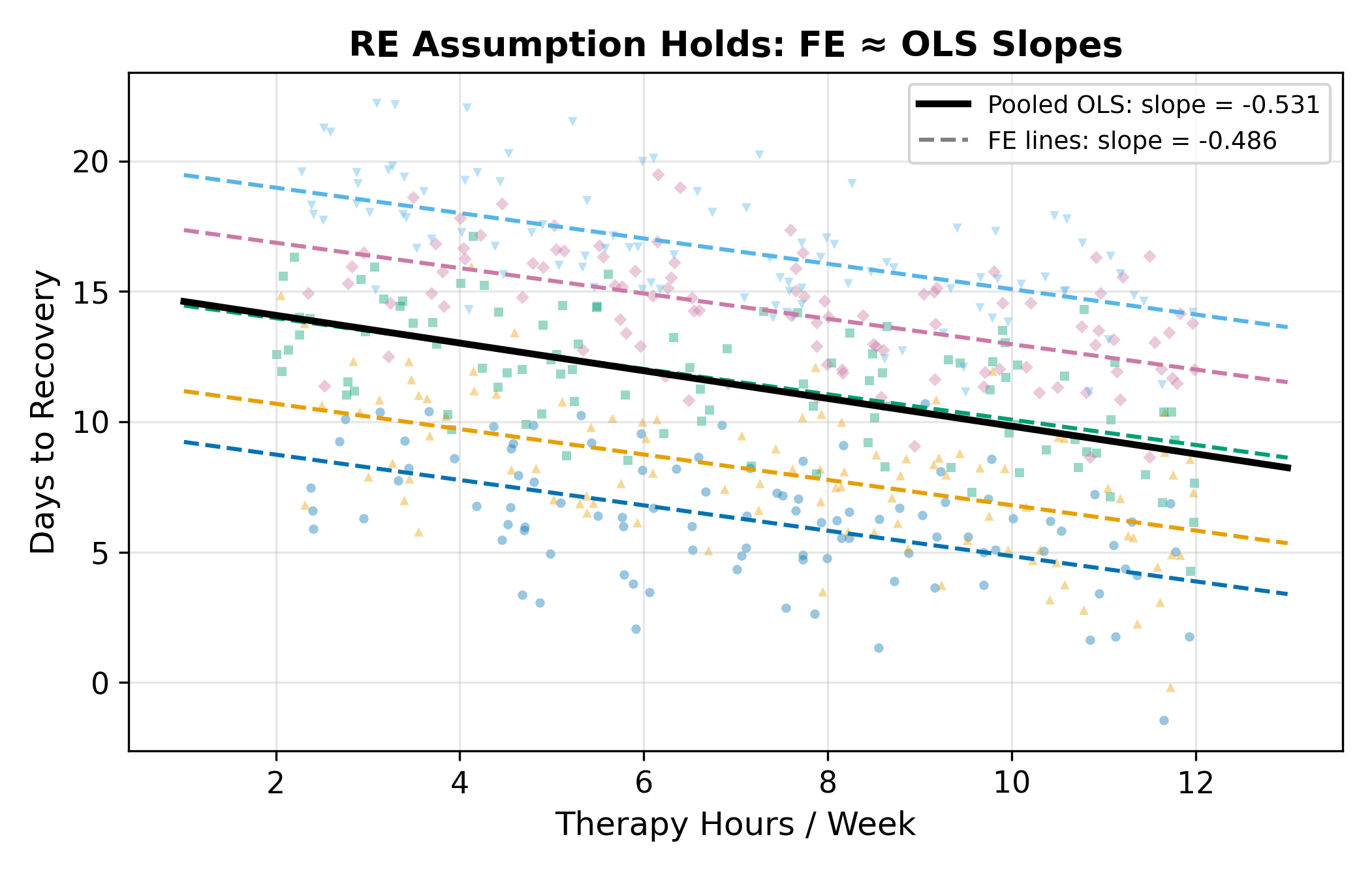
10.5.1 The Spectrum from OLS to FE
What makes RE elegant is that the partial demeaning nests both pooled OLS and fixed effects as limiting cases. The value of \(\hat\alpha\) controls where you land on the spectrum:
| \(\hat\alpha\) | Transformation | Equivalent to |
|---|---|---|
| \(0\) | \(y_{ij} - 0 \cdot \bar y_j = y_{ij}\) | Pooled OLS (no group adjustment) |
| Between 0 and 1 | \(y_{ij} - \hat\alpha_j \bar y_j\) | RE (weighted mix of within and between) |
| \(1\) | \(y_{ij} - \bar y_j\) | FE (full within demeaning) |
What pushes \(\hat\alpha\) toward 1 (so RE behaves like FE)?
- Large \(\sigma_u^2\) relative to \(\sigma_e^2\). When between-group variance dominates, you want full demeaning, the group effects are doing all the work and you should sweep them out completely.
- Large \(N_j\). With many observations per group, each group’s mean is a precise estimate of its own baseline, and you don’t need to borrow from the ensemble.
What pushes \(\hat\alpha\) toward 0 (so RE behaves like pooled OLS)?
- Small \(\sigma_u^2\). When hospitals look basically alike, there’s no group effect worth controlling for.
- Small \(N_j\). With one or two observations per group, you can’t trust the local mean and must lean on the ensemble.
In a typical applied panel, \(\hat\alpha\) comes out somewhere in the middle, anywhere from \(0.3\) to \(0.9\) is common. The partial demeaning extracts most of the FE protection while keeping some of the between-group information.
10.6 When to Use RE vs FE
This is the modeling decision the chapter has been building toward. It comes down to whether you can defend the RE assumption \(\operatorname{Cov}(u_j, x_{ij}) = 0\).
10.6.1 When RE Is the Right Call
- The groups are random draws from a larger population. You sampled 200 hospitals from a registry of 5,000. The groups in your data are interchangeable with groups you didn’t sample. The population-level distribution \(u_j \sim (0, \sigma_u^2)\) is meaningful.
- There is no specific reason to think group effects correlate with the regressor of interest. Random assignment is the gold standard; natural experiments or quasi-experimental designs that approximate random assignment work too.
- You need to estimate the effect of a time-invariant (group-level) variable. Teaching-hospital status, urban vs. rural, country institutions, anything that doesn’t change within group. FE makes these invisible; only RE can estimate them.
- Efficiency matters. RE uses both within- and between-group variation, so it has smaller standard errors than FE when the RE assumption holds. With small samples or weak within-group variation, this efficiency gain can be substantial.
10.6.2 When FE Is the Safer Call
- Groups are specific entities you care about, not a random draw. These five particular hospitals, these 50 specific countries. The population-level distribution of \(u_j\) doesn’t quite make sense; you’re not generalizing to “hospitals in general.”
- Plausible correlation between group effects and the regressor. Better hospitals may push more aggressive protocols. Larger firms may invest more. Older countries may have different growth patterns. If you can tell a story for why \(\operatorname{Cov}(u_j, x_{ij}) \neq 0\), FE is safer.
- Micro data with individuals or firms. Unobserved ability, management quality, taste, these almost always correlate with the things people choose to do (education, training, hiring). FE is the conservative default.
- You only care about within-group effects. “Among patients at the same hospital, does more therapy help?” That’s exactly what FE estimates. RE answers a slightly different question (within and between combined), which may or may not be what you want.
When in doubt, FE is the conservative choice. RE is the reward for being able to defend the exogeneity assumption.
10.7 The Hausman Test
The decision between FE and RE has a formal statistical version: the Hausman test. It compares the FE and RE estimates of \(\beta\) and asks whether the difference is large enough to reject the RE assumption.
10.7.1 The Logic
Under the RE assumption \(\operatorname{Cov}(u_j, x_{ij}) = 0\):
- FE is consistent (\(\hat\beta^{\text{FE}} \to \beta\)).
- RE is also consistent (\(\hat\beta^{\text{RE}} \to \beta\)).
- RE is more efficient than FE (smaller variance).
So when the RE assumption holds, \(\hat\beta^{\text{FE}}\) and \(\hat\beta^{\text{RE}}\) are both estimating the same number, and they should agree closely.
When the RE assumption fails:
- FE is still consistent.
- RE is inconsistent, the partial demeaning leaves a residual correlation between the transformed regressors and the transformed errors.
- The two estimates point at different numbers and the gap stays open as the sample grows.
The Hausman test puts this on a statistical footing: take the difference and see if it is too large to be sampling noise.
10.7.2 The Test Statistic
For a single regressor, the test statistic is
\[ H = \frac{\hat\beta^{\text{FE}} - \hat\beta^{\text{RE}}}{\sqrt{\widehat{\operatorname{Var}}(\hat\beta^{\text{FE}}) - \widehat{\operatorname{Var}}(\hat\beta^{\text{RE}})}}. \tag{10.8}\]
Under the RE assumption, \(H\) is approximately standard normal in large samples. With multiple regressors, the test generalizes to a \(\chi^2\) statistic with degrees of freedom equal to the number of regressors. Stata, R’s plm, and Python’s linearmodels all compute it automatically.
The denominator is well-defined because, under the RE assumption, RE is more efficient than FE: \(\operatorname{Var}(\hat\beta^{\text{FE}}) > \operatorname{Var}(\hat\beta^{\text{RE}})\), so the difference under the square root is positive.
10.7.3 The Decision Rule
| Result | Interpretation | Action |
|---|---|---|
| Reject \(H_0\) (\(p < 0.05\)) | FE and RE disagree more than chance allows. RE is inconsistent. | Use FE. |
| Fail to reject (\(p \geq 0.05\)) | FE and RE agree within sampling error. RE assumption is reasonable. | Use RE (more efficient). |
In one slogan: FE is safe; RE is the reward for being able to justify the exogeneity assumption. If you can convince a referee that \(\operatorname{Cov}(u_j, x_{ij}) = 0\), RE gives you tighter standard errors and access to time-invariant covariates. If you can’t, FE has your back.
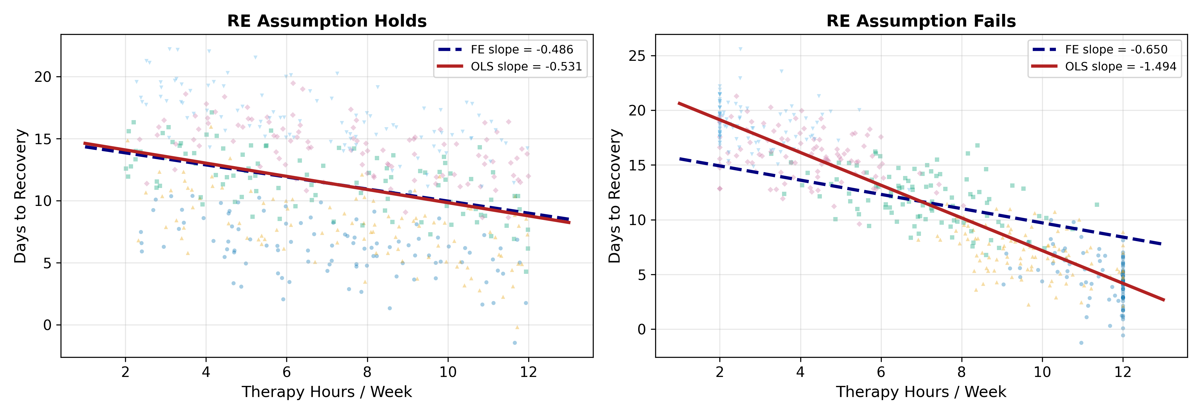
10.7.4 Worked Example: Hospital Recovery Data
Run both estimators on the hospital data:
| FE | RE | |
|---|---|---|
| Slope \(\hat\beta\) on therapy hours | \(-0.500\) | \(-0.497\) |
| \(\widehat{\operatorname{Var}}(\hat\beta)\) | \(0.00180\) | \(0.00165\) |
The two slopes are nearly identical (a difference of \(0.003\)). The variance of FE is slightly larger, as the theory predicts when RE is consistent.
The Hausman statistic:
\[ H = \frac{-0.500 - (-0.497)}{\sqrt{0.00180 - 0.00165}} = \frac{-0.003}{\sqrt{0.00015}} = \frac{-0.003}{0.0122} \approx -0.25. \]
The absolute value is \(0.25\), well below the critical value \(1.96\) for a two-sided 5% test. Fail to reject \(H_0\). The RE assumption holds within sampling error, so RE is the right call, and it’s the more efficient one.
If the FE slope had come out at \(-0.45\) instead (with the same variances), the Hausman statistic would be \(-0.45 - (-0.497) = 0.047\) divided by \(0.0122\) which is \(3.85\). That would reject decisively, and we would conclude that hospital quality is correlated with therapy hours after all. FE would be the right call.
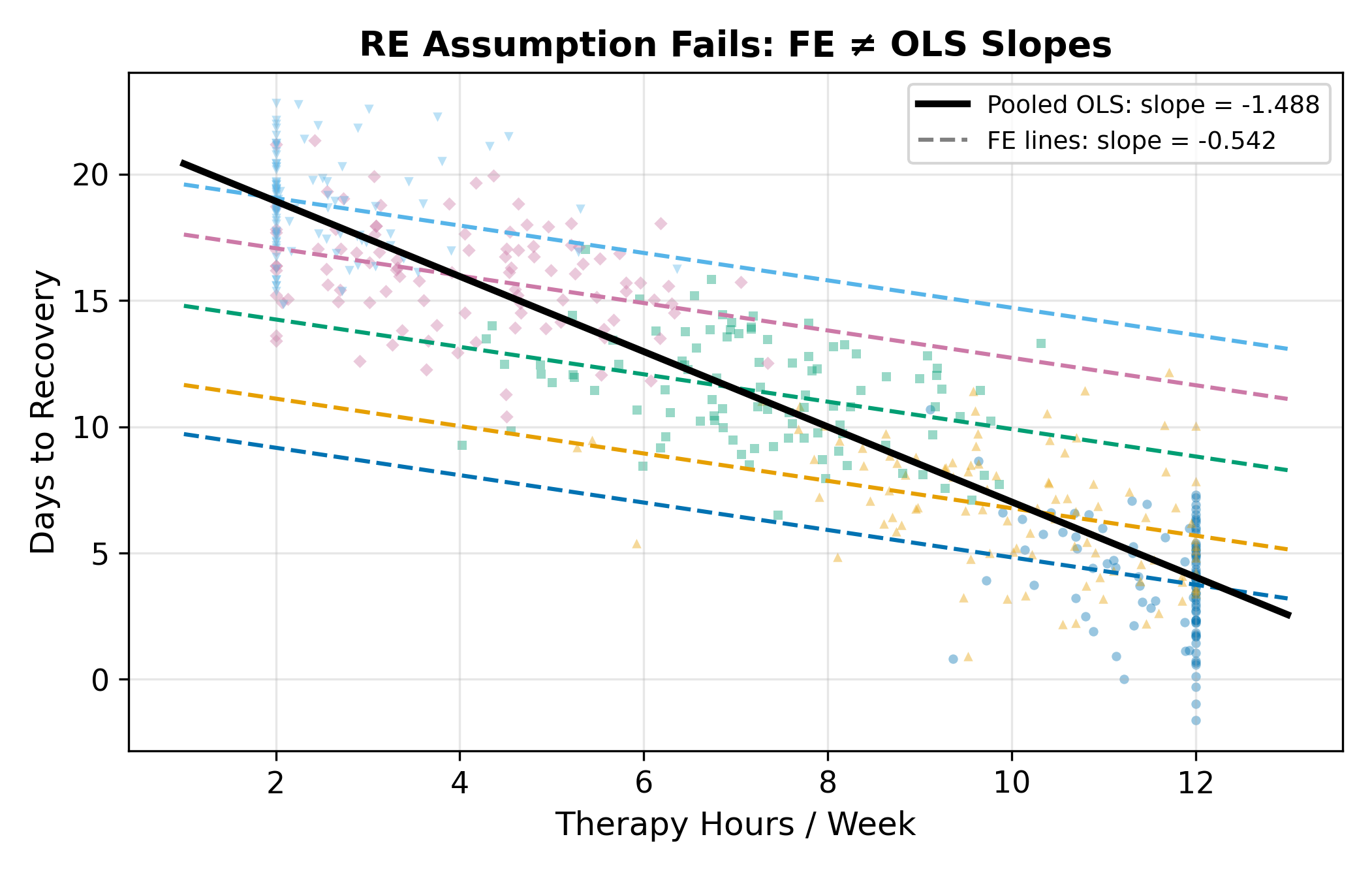
\(H = 4.2\) is well above \(1.96\), so reject \(H_0\). The FE and RE estimates disagree more than sampling noise allows. Mechanically, that means \(\operatorname{Cov}(u_j, x_{ij}) \neq 0\): hospitals with different unobserved quality systematically administer different amounts of therapy. The story could be either direction (better hospitals push more therapy, or sicker patients at better hospitals get more therapy), but the test only tells you that there is a correlation, not which way it points.
Either way, RE is inconsistent and you should report FE.
10.8 A Decision Flowchart
Put it all together:
- Is there unobserved group heterogeneity at all? If no, pooled OLS is fine. If yes, continue.
- Do you need to estimate the effect of a time-invariant group-level variable? If yes, you must use RE (or a hybrid like Hausman-Taylor), FE would absorb the variable.
- Is \(\operatorname{Cov}(u_j, x_{ij}) = 0\) plausible on theoretical grounds? If clearly not, use FE. If maybe, run the Hausman test.
- Hausman test result? Reject \(\implies\) FE. Fail to reject \(\implies\) RE.
Step 3 is the modeling step that no statistical procedure can do for you. The Hausman test in step 4 is informative but not all-powerful: it has low power against small violations of the assumption, and it conflates the RE assumption with other modeling choices (functional form, etc.). Most applied papers report FE as the headline specification and note that RE gives similar results, that combination is the most defensible position when you can manage it.
10.9 What’s Next
- Cluster-Robust SEs handle the inference problem (correlated within-group residuals) that motivated RE in the first place, but with a much weaker assumption than RE.
- Hausman-Taylor is a hybrid that allows some time-invariant variables to enter while still controlling for FE-style unobserved heterogeneity in others.
- Dynamic Panels handles the case where \(y_{i,t-1}\) is a regressor.