4  Measurement Error

Attenuation Bias and the Reliability Ratio

NotePrerequisites

This chapter assumes familiarity with OLS estimation and omitted variable bias. For the instrumental variables solution, see Instrumental Variables.

4.1 Motivation

The errors-in-variables problem occurs when an explanatory variable is measured with error. If we measure an explanatory variable with error, then it is correlated with the error term, and the least squares estimator is inconsistent.

4.1.1 Example: Study Time and Test Scores

Suppose that test scores (\(y_i\)) depend on true study time (\(x_i^*\)):

\[ y_i = \beta_1 + \beta_2 x_i^* + v_i \]

We measure test scores precisely, but we don’t observe true study time. Instead, we only have data on office hours attendance (\(x_i\)), which is a noisy proxy for total study time. Some students study a lot but never come to office hours; others show up frequently but don’t study much otherwise.

We model this measurement error as:

\[ x_i = x_i^* + u_i \]

where \(u_i\) is the measurement error with mean 0 and variance \(\sigma_u^2\). Assume \(u_i\) is independent of the regression error \(v_i\).

4.2 Why Measurement Error Causes Endogeneity

When we substitute \(x_i^* = x_i - u_i\) into the true model:

\[ y_i = \beta_1 + \beta_2(x_i - u_i) + v_i = \beta_1 + \beta_2 x_i + (v_i - \beta_2 u_i) \]

Let \(e_i = v_i - \beta_2 u_i\) be the composite error. Now check exogeneity:

\[ \text{Cov}(x_i, e_i) = \text{Cov}(x_i^* + u_i, v_i - \beta_2 u_i) = E\left[(x_i^* + u_i)(v_i - \beta_2 u_i)\right] \]

Since \(x_i^*\) is exogenous (\(E(x_i^* v_i) = 0\)) and \(u_i\) is independent of \(v_i\):

\[ \text{Cov}(x_i, e_i) = E(-\beta_2 u_i^2) = -\beta_2 \sigma_u^2 \neq 0 \]

If \(\beta_2 > 0\), there is a negative correlation between \(x_i\) and \(e_i\). OLS underestimates \(\beta_2\).

4.3 Attenuation Bias Formula

As the sample size \(N\) gets larger, the OLS estimator \(b_2\) moves toward the following expression:

\[ \beta_2 \cdot \frac{\sigma_{x^*}^2}{\sigma_{x^*}^2 + \sigma_u^2} = \beta_2 \cdot \lambda \]

where \(\lambda = \frac{\sigma_{x^*}^2}{\sigma_{x^*}^2 + \sigma_u^2}\) is called the reliability ratio (always between 0 and 1).

• If \(\sigma_u^2 = 0\) (no measurement error): \(\lambda = 1\) and \(b_2 \to \beta_2\) ✓
• If \(\sigma_u^2 \to \infty\) (pure noise): \(\lambda \to 0\) and \(b_2 \to 0\)

This is called attenuation bias—measurement error biases the coefficient toward zero, and more data won’t fix it.

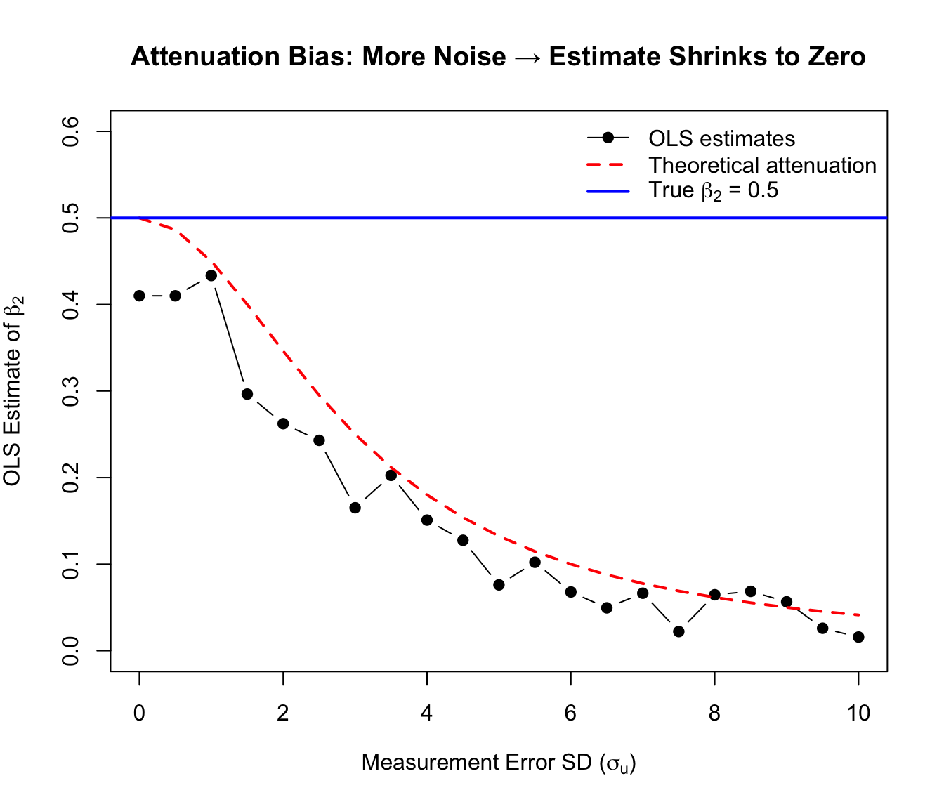
4.4 Simulation: Watching Attenuation Bias in Action

set.seed(123)
n <- 500
beta_true <- 0.5

# True study time (unobserved)
x_star <- rnorm(n, mean = 10, sd = 3)

# Test scores
y <- 50 + beta_true * x_star + rnorm(n, sd = 5)

# Vary measurement error variance
sigma_u_values <- seq(0, 10, by = 0.5)
estimates <- numeric(length(sigma_u_values))

for (i in seq_along(sigma_u_values)) {
  sigma_u <- sigma_u_values[i]
  # Observed proxy (office hours attendance) = true study time + noise
  x_observed <- x_star + rnorm(n, sd = sigma_u)
  estimates[i] <- coef(lm(y ~ x_observed))[2]
}

# Theoretical attenuation
sigma_x_star <- 3
lambda <- sigma_x_star^2 / (sigma_x_star^2 + sigma_u_values^2)
theoretical <- beta_true * lambda

# Plot
plot(sigma_u_values, estimates, type = "b", pch = 19,
     xlab = expression(paste("Measurement Error SD (", sigma[u], ")")),
     ylab = expression(paste("OLS Estimate of ", beta[2])),
     ylim = c(0, 0.6),
     main = "Attenuation Bias: More Noise → Estimate Shrinks to Zero")
lines(sigma_u_values, theoretical, col = "red", lwd = 2, lty = 2)
abline(h = beta_true, col = "blue", lwd = 2)
legend("topright",
       legend = c("OLS estimates", "Theoretical attenuation",
                  expression(paste("True ", beta[2], " = 0.5"))),
       pch = c(19, NA, NA), lty = c(1, 2, 1), lwd = c(1, 2, 2),
       col = c("black", "red", "blue"), bty = "n")

As measurement error increases, the OLS estimate shrinks toward zero

WarningThe Intuition

When office hours attendance is mostly noise (high \(\sigma_u^2\)), it tells us almost nothing about true study time. If the regressor contains no real information, it can’t predict test scores—so the estimated coefficient collapses to zero.

4.5 Slide Deck

Slides

Download slides (PDF)

Presentation

Download presentation slides (with transitions) (PDF)

TipWhat’s next?

When a regressor is endogenous (whether from OVB, measurement error, or simultaneity), Instrumental Variables provide a way to recover causal estimates. For panel data approaches to endogeneity, see Fixed Effects.