17 Multinomial Logit
Modeling Unordered Choices Among Multiple Alternatives
When individuals choose among three or more unordered alternatives (bus, train, car), separate binary logits fail because they ignore the full choice set. Multinomial logit uses a softmax probability across all alternatives. Conditional logit extends this to alternative-specific variables like travel time and cost. Both rest on the Independence of Irrelevant Alternatives assumption.
This page extends the binary logit framework from the Qualitative and Limited Dependent Variable Models hub. You should be comfortable with latent variables, the logistic CDF, maximum likelihood estimation, and marginal effects before continuing.
17.1 The Problem: More Than Two Choices
Binary logit handles yes/no decisions: work or not, default or not, drive or take the bus. But many economic decisions involve choosing from three or more unordered alternatives. A commuter picks among bus, train, and car. A student selects a college major. A consumer chooses between brands.
A natural first attempt is to run separate binary logits for each pair: bus vs. car, train vs. car, bus vs. train. This fails for two reasons:
- Probabilities don’t sum to one. Three separate binary models produce three independent probability estimates. Nothing constrains \(P(\text{bus}) + P(\text{train}) + P(\text{car}) = 1\). You can easily end up with total probability above or below one.
- Each model ignores the full choice set. The bus-vs-car logit treats the data as if train doesn’t exist. But adding a train option should change the probability of choosing bus or car.
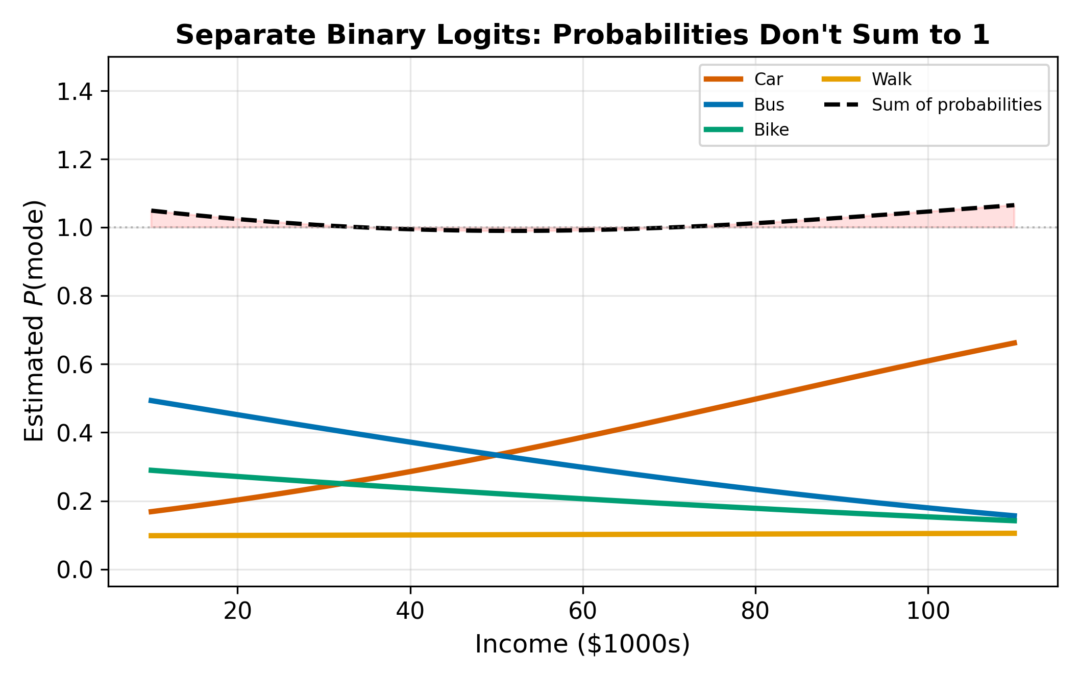
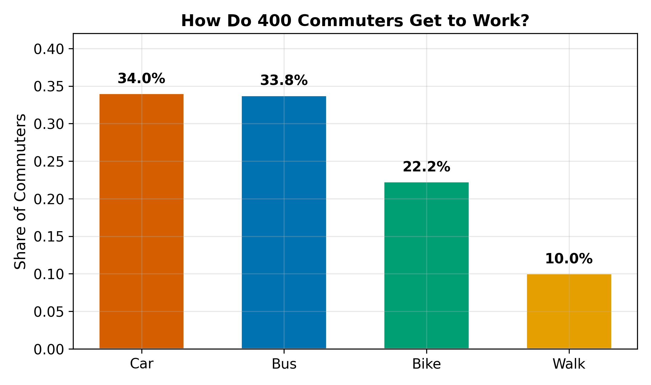
The data tell the same story. Suppose we observe 1,000 commuters: 400 choose car, 350 choose bus, 250 choose train. These shares reflect the full choice environment. Any model that doesn’t respect the complete set of alternatives is throwing away information.
The “probabilities must sum to one” constraint is not just bookkeeping. It encodes the economic idea that if one alternative becomes more attractive, the others must lose share.
\(\implies\) We need a single model that simultaneously assigns probabilities to all alternatives, with the constraint that they sum to one.
17.2 Multinomial Logit
17.2.1 Random Utility Foundation
The multinomial logit (MNL) model starts from a random utility framework. Individual \(i\) gets utility from choosing alternative \(j\):
\[ U_{ij} = V_{ij} + \varepsilon_{ij} \tag{17.1}\]
where \(V_{ij}\) is the systematic (observable) component and \(\varepsilon_{ij}\) is a random (unobservable) component. The individual chooses the alternative that maximizes utility. If the \(\varepsilon_{ij}\) terms follow independent Type I Extreme Value (Gumbel) distributions, the choice probabilities take the softmax form:
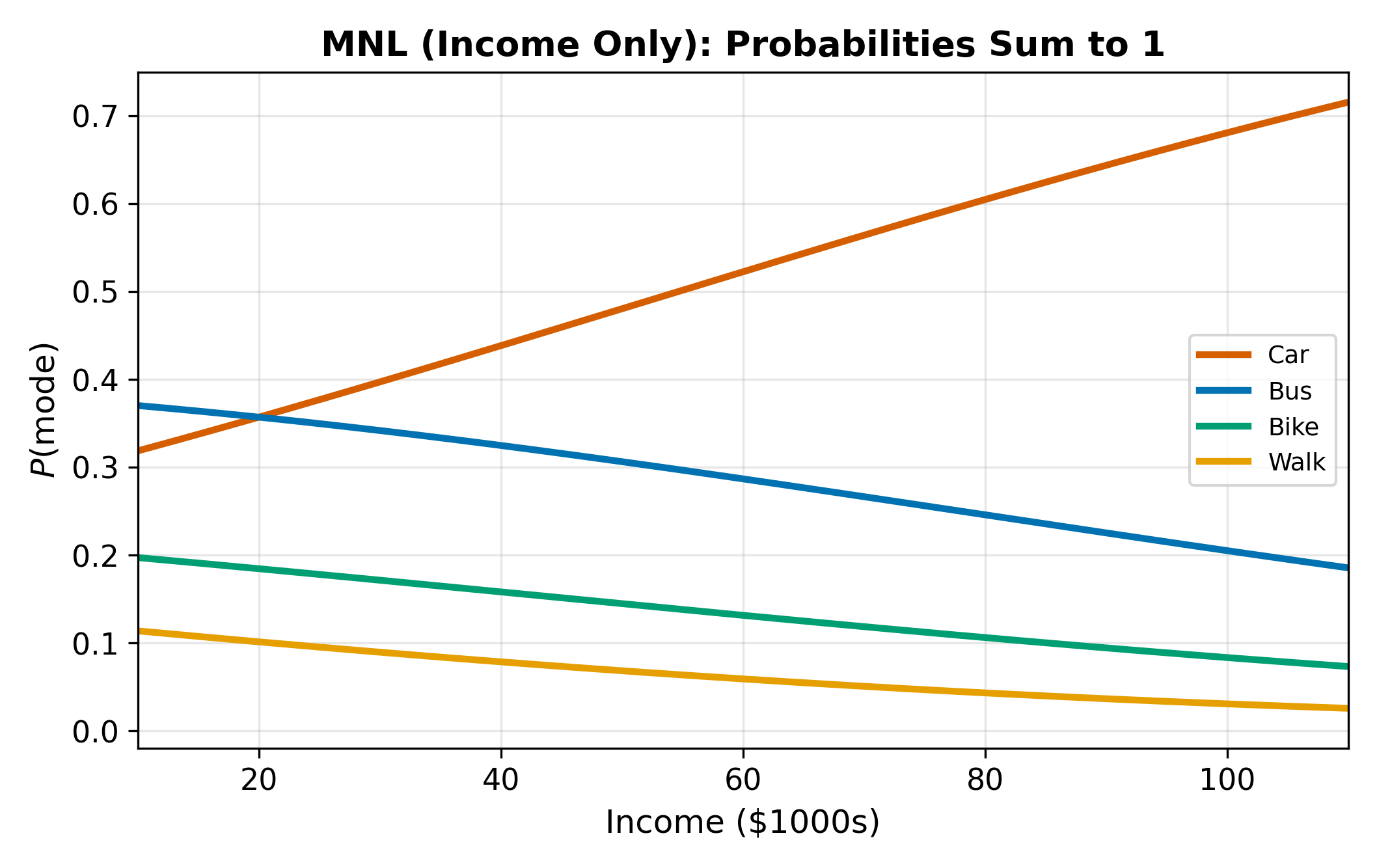
\[ P(y_i = j) = \frac{e^{V_{ij}}}{\sum_{k=1}^{J} e^{V_{ik}}} \tag{17.2}\]
This is the multinomial logit probability. The denominator sums over all \(J\) alternatives, guaranteeing that probabilities sum to one. Each probability is strictly between 0 and 1.
17.2.2 Individual-Specific Variables
In the standard MNL setup, the explanatory variables describe the individual, not the alternative. Income, age, and education are the same no matter which mode the commuter is evaluating. The systematic utility is:
\[ V_{ij} = \alpha_j + \boldsymbol{\beta}_j' \mathbf{x}_i \tag{17.3}\]
Each alternative \(j\) gets its own intercept \(\alpha_j\) and its own coefficient vector \(\boldsymbol{\beta}_j\). This is what makes MNL different from binary logit with a single set of coefficients: the effect of income on choosing bus can differ from its effect on choosing train.
Why does each alternative get its own \(\boldsymbol{\beta}_j\)? Because the same individual characteristic can push toward different alternatives. Higher income might increase car probability but decrease bus probability. A single \(\beta\) cannot capture both directions.
17.2.3 Normalization
The softmax probability in Equation 17.2 depends only on differences in utility. Adding a constant \(c\) to every \(V_{ij}\) leaves the probabilities unchanged:
\[ \frac{e^{V_{ij} + c}}{\sum_k e^{V_{ik} + c}} = \frac{e^c \cdot e^{V_{ij}}}{e^c \cdot \sum_k e^{V_{ik}}} = \frac{e^{V_{ij}}}{\sum_k e^{V_{ik}}} \]
This means one alternative’s parameters are redundant. We normalize by setting the coefficients for one base category to zero: \(\alpha_1 = 0\), \(\boldsymbol{\beta}_1 = \mathbf{0}\). The remaining \(J - 1\) sets of coefficients measure utility relative to the base.
The choice of base category affects the coefficients but not the predicted probabilities or marginal effects. Switching the base rescales the \(\alpha_j\) and \(\boldsymbol{\beta}_j\) values, but the model fit is identical. Pick whichever base makes interpretation easiest.
With the base category normalization and \(J = 3\) alternatives, the probabilities become:
\[ P(y_i = 1) = \frac{1}{1 + e^{V_{i2}} + e^{V_{i3}}}, \quad P(y_i = j) = \frac{e^{V_{ij}}}{1 + e^{V_{i2}} + e^{V_{i3}}} \quad \text{for } j = 2, 3 \tag{17.4}\]
When \(J = 2\), this collapses to the binary logit model from the hub page.
17.2.4 Estimation
Like binary logit, MNL is estimated by maximum likelihood. Each observation contributes to the log-likelihood based on which alternative was actually chosen:
\[ \ln L = \sum_{i=1}^{N} \sum_{j=1}^{J} d_{ij} \ln P(y_i = j) \tag{17.5}\]
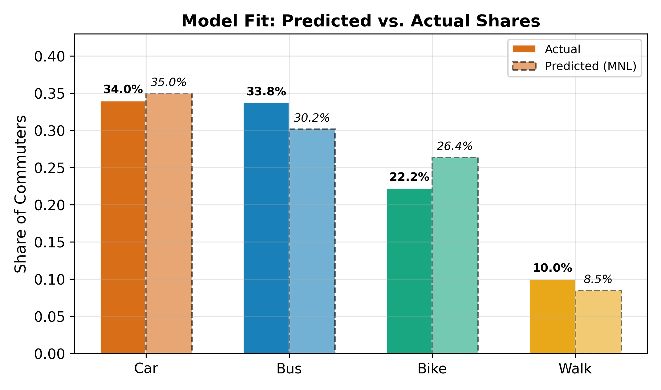
where \(d_{ij} = 1\) if individual \(i\) chose alternative \(j\) and 0 otherwise. The optimizer searches over all the \(\alpha_j\) and \(\boldsymbol{\beta}_j\) parameters simultaneously. With \(J\) alternatives and \(K\) regressors, you estimate \((J-1)(K+1)\) parameters. The parameter count grows quickly: 3 alternatives with 4 regressors means 10 parameters; 5 alternatives with 4 regressors means 20.
\(\implies\) Report marginal effects or predicted probabilities rather than raw coefficients. With so many parameters, a table of \(\hat{\beta}_{jk}\) values is difficult for readers to digest.
17.3 Interpreting MNL Coefficients
17.3.1 Log-Odds Ratios
The MNL coefficients have a direct interpretation as log-odds ratios relative to the base. Taking the ratio of \(P(y_i = j)\) to \(P(y_i = 1)\):
\[ \ln \frac{P(y_i = j)}{P(y_i = 1)} = \alpha_j + \boldsymbol{\beta}_j' \mathbf{x}_i \tag{17.6}\]
A one-unit increase in \(x_k\) changes the log-odds of choosing alternative \(j\) over the base by \(\beta_{jk}\). This is clean but limited: it tells you about the relative odds of two specific alternatives, not how the full set of probabilities shifts.
17.3.2 Marginal Effects
For policy analysis, marginal effects are more useful. The marginal effect of \(x_k\) on the probability of choosing alternative \(j\) is:
\[ \frac{\partial P(y_i = j)}{\partial x_k} = P(y_i = j) \left[ \beta_{jk} - \sum_{m=1}^{J} P(y_i = m) \, \beta_{mk} \right] \tag{17.7}\]
where \(\beta_{1k} = 0\) (the base category coefficient). Three things to notice:
- The marginal effect depends on all the probabilities and all the coefficients, not just those for alternative \(j\).
- The marginal effect varies across observations because the probabilities \(P(y_i = j)\) vary.
- Marginal effects for a given \(x_k\) always sum to zero across alternatives: if income makes car more likely, bus and train must become less likely by exactly the offsetting amount.
Because probabilities must sum to one: \(\sum_j P(y_i = j) = 1\). Differentiate both sides with respect to \(x_k\):
\[ \sum_{j=1}^{J} \frac{\partial P(y_i = j)}{\partial x_k} = 0 \]
Any probability that goes up must be exactly offset by probabilities that go down. This constraint is automatic in the MNL model. It would be violated by running separate binary logits, which is another reason the pairwise approach fails.
17.4 Conditional Logit
17.4.1 Alternative-Specific Variables
The standard MNL uses variables that describe the individual (\(x_i\)): income, age, education. But many choice problems involve variables that describe the alternatives: the travel time of each mode, the price of each brand, the tuition of each university. These variables vary across both individuals and alternatives.
The conditional logit model (McFadden, 1974) handles alternative-specific variables. The systematic utility becomes:
\[ V_{ij} = \beta_{\text{time}} \cdot \text{Time}_{ij} + \beta_{\text{cost}} \cdot \text{Cost}_{ij} \tag{17.8}\]
The coefficients \(\beta_{\text{time}}\) and \(\beta_{\text{cost}}\) are the same for all alternatives. This makes sense: an extra minute of travel time is equally unpleasant whether it’s on the bus or the train. The variation comes from the fact that \(\text{Time}_{ij}\) differs across modes.
Terminology can be confusing. Some textbooks call the individual-specific-variable model “multinomial logit” and the alternative-specific-variable model “conditional logit.” Others use “multinomial logit” for both. The distinction that matters is whether the coefficients vary across alternatives (\(\boldsymbol{\beta}_j\)) or are constant (\(\boldsymbol{\beta}\)).
17.4.2 The Combined Model
In practice, most applications include both types of variables. The combined specification is:
\[ V_{ij} = \alpha_j + \boldsymbol{\beta}_j' \mathbf{x}_i + \boldsymbol{\gamma}' \mathbf{z}_{ij} \tag{17.9}\]
where \(\mathbf{x}_i\) are individual-specific variables (with alternative-specific coefficients \(\boldsymbol{\beta}_j\)) and \(\mathbf{z}_{ij}\) are alternative-specific variables (with common coefficients \(\boldsymbol{\gamma}\)). The choice probabilities still follow the softmax formula in Equation 17.2.
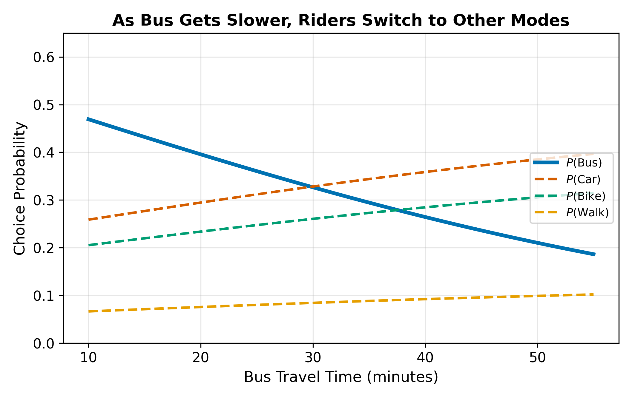
For the transportation example: income affects mode choice differently for each mode (higher income increases car probability more than bus probability), while travel time affects all modes in the same direction (longer time reduces choice probability).
\(\implies\) The combined model is the workhorse of applied discrete choice analysis. Pure MNL (individual variables only) cannot explain why someone switches from bus to car when bus fares rise. Pure conditional logit (alternative variables only) cannot explain why high-income individuals prefer car regardless of travel times. The combined model handles both.
17.5 Independence of Irrelevant Alternatives
17.5.1 The IIA Property
The ratio of choice probabilities for any two alternatives depends only on those two alternatives:
\[ \frac{P(y_i = j)}{P(y_i = k)} = \frac{e^{V_{ij}}}{e^{V_{ik}}} = e^{V_{ij} - V_{ik}} \tag{17.10}\]
No other alternative appears in this expression. Adding or removing a third option from the choice set does not change the relative odds of \(j\) vs. \(k\). This is the Independence of Irrelevant Alternatives (IIA) property.
IIA follows directly from the assumption that the random errors \(\varepsilon_{ij}\) are independent across alternatives. If my preference shock for the bus is unrelated to my preference shock for the train, then learning about a new option shouldn’t change the bus/train comparison.
In many settings IIA is reasonable. If the alternatives are genuinely distinct (different product categories, different industries, different career paths), there is no reason to expect correlated unobservables. The problems arise when alternatives share unobserved attributes.
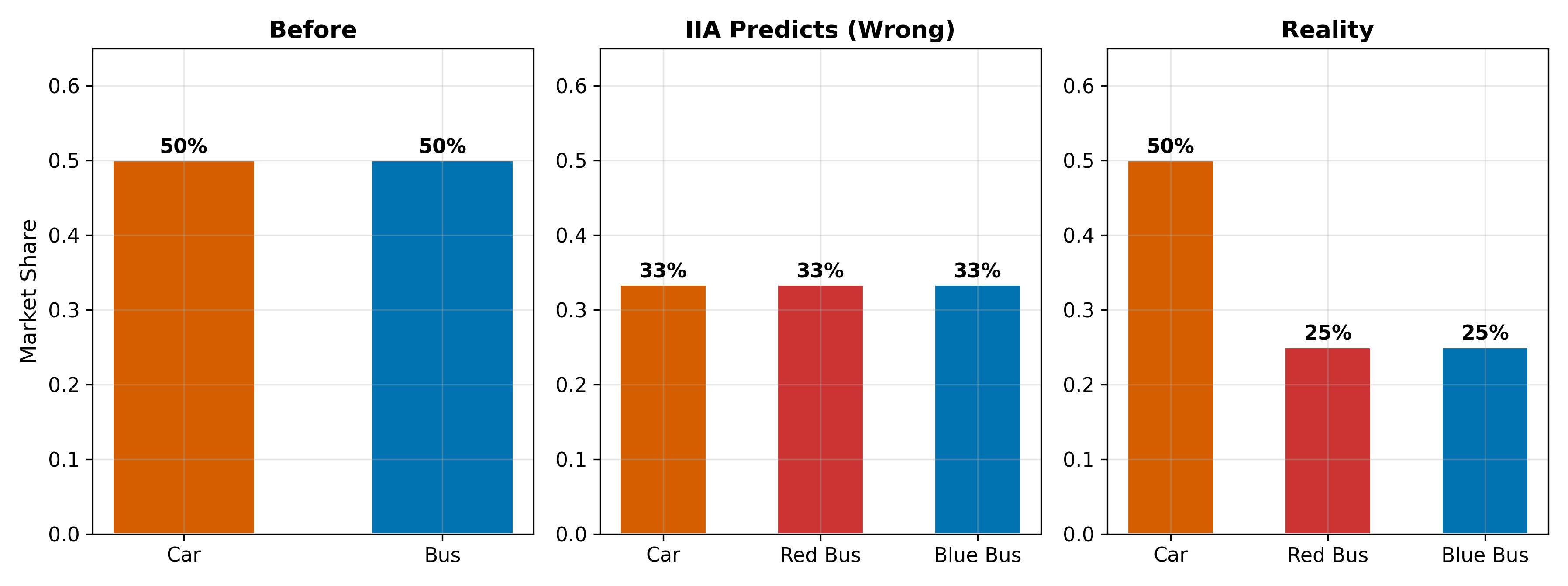
17.5.2 The Red Bus / Blue Bus Problem
The classic illustration of IIA failure:
A city has two transportation modes with equal market share:
\[ P(\text{car}) = 0.5, \quad P(\text{red bus}) = 0.5 \]
Now the city introduces a blue bus that is identical to the red bus in every respect except color. Intuitively, the blue bus should split the bus market:
\[ P(\text{car}) = 0.5, \quad P(\text{red bus}) = 0.25, \quad P(\text{blue bus}) = 0.25 \]
But IIA forces the original ratio to be preserved. Since \(P(\text{car}) / P(\text{red bus}) = 1\) before, IIA requires it to stay at 1 after:
\[ P(\text{car}) = 0.33, \quad P(\text{red bus}) = 0.33, \quad P(\text{blue bus}) = 0.33 \]
The model predicts that adding a clone of an existing option draws equally from all alternatives, including the completely unrelated car. This is absurd. The problem is that red bus and blue bus are close substitutes, violating the independence assumption on which IIA rests.
IIA is testable via the Hausman-McFadden test: drop one alternative, re-estimate, and check whether the remaining coefficients change significantly. A large change suggests IIA is violated.
17.5.3 When IIA Fails
IIA is violated whenever some alternatives are closer substitutes than others. Common examples:
- Transportation: Bus and train are closer substitutes than bus and car (both are public transit).
- Brand choice: Store brands compete more with each other than with premium brands.
- Residential location: Neighborhoods in the same district are closer substitutes than neighborhoods across the city.
When IIA fails, three alternatives to MNL are available:
| Model | What it does | Cost |
|---|---|---|
| Nested logit | Groups similar alternatives into nests; IIA holds within nests but not across | Must specify the nesting structure |
| Mixed logit | Allows coefficients to vary randomly across individuals | Computationally intensive; simulation-based |
| Multinomial probit | Uses a full covariance matrix for the errors | Very computationally demanding; rarely used in practice |
Consider college choice among UCLA, UC Berkeley, Stanford, and a community college. UCLA and Berkeley are close substitutes (similar public universities, similar cost, similar prestige). If Berkeley suddenly became much harder to get into, its lost applicants would mostly shift to UCLA, not to the community college. But IIA would predict equal proportional shifts to all remaining alternatives. Nested logit with a “UC system” nest and a “non-UC” nest would handle this correctly.
Count Data Models covers the Poisson and negative binomial models for non-negative integer outcomes, where the dependent variable counts events (doctor visits, patents, arrests) rather than selecting among categories.