15 Binary Choice Models
LPM, Logit, and Probit for Yes/No Outcomes
When the outcome is binary (admitted/rejected, employed/unemployed), OLS can produce impossible predictions and biased marginal effects. Logit and probit models constrain predicted probabilities to [0, 1] through an S-shaped link function. This page builds the intuition visually, from the LPM’s failures through the latent variable framework to marginal effects interpretation.
This page is part of the Qualitative and Limited Dependent Variable Models sequence. You should be comfortable with OLS regression and the idea of conditional expectation before reading.
15.1 The Linear Probability Model
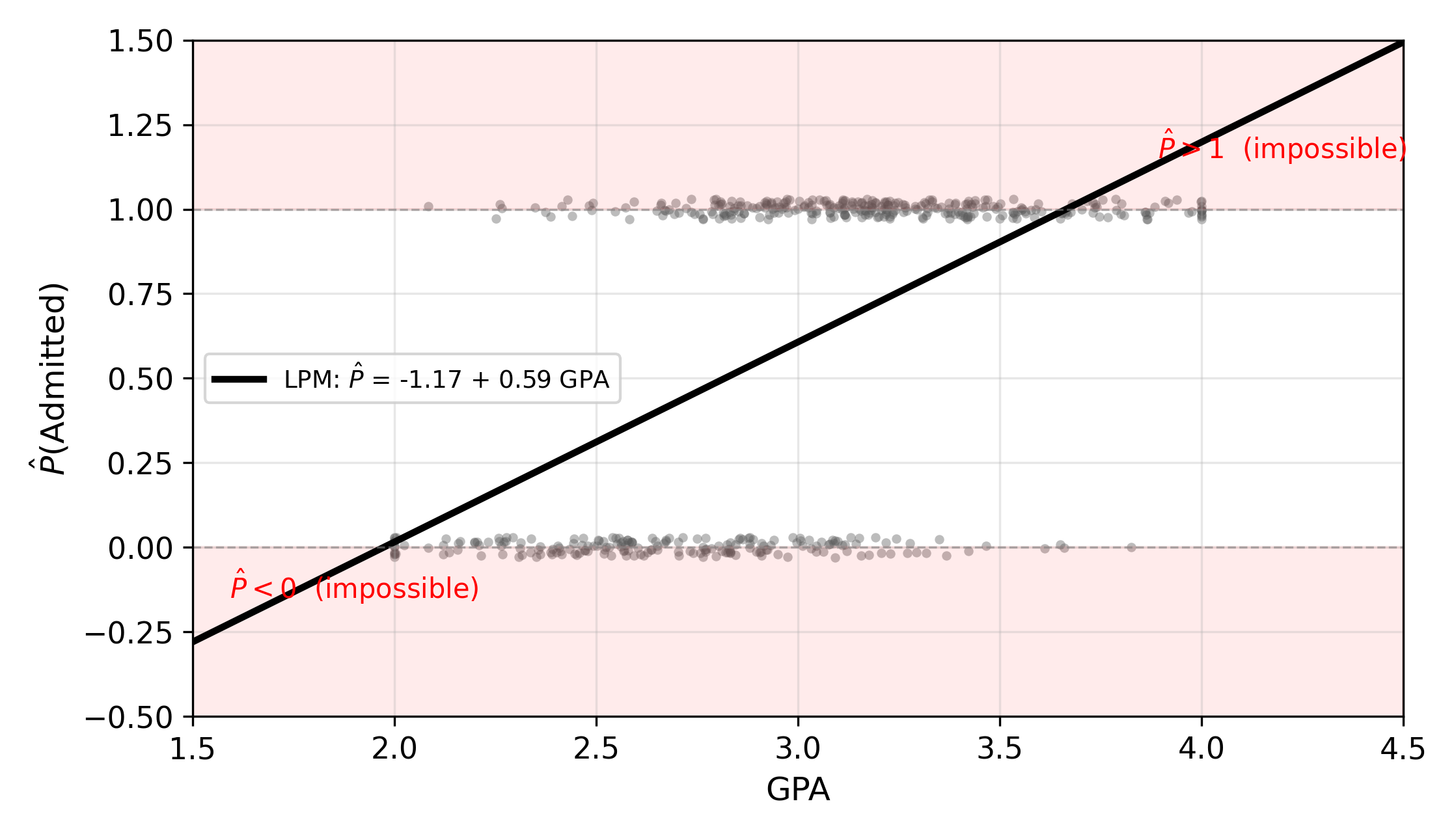
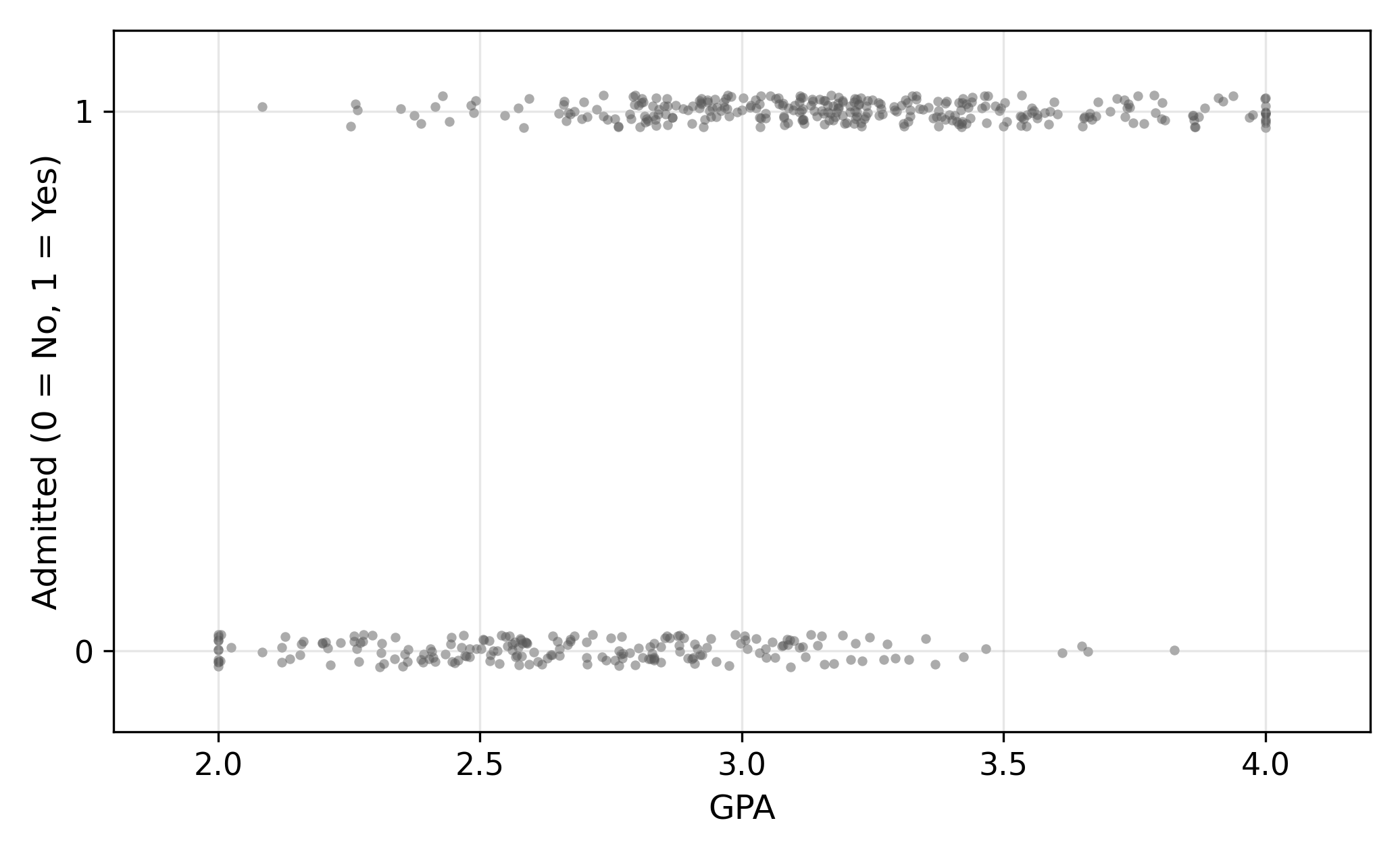
Suppose we want to predict whether a student is admitted to a graduate program (\(\text{Admit}_i = 1\)) or rejected (\(\text{Admit}_i = 0\)) based on their undergraduate GPA. The most natural starting point is to just run OLS:
\[ P(\text{Admit}_i = 1 \mid \text{GPA}_i) = \beta_0 + \beta_1 \, \text{GPA}_i \tag{15.1}\]
This is the linear probability model (LPM). The fitted values \(\hat{y}_i\) are interpreted as predicted probabilities of admission.
The LPM is easy to estimate and easy to interpret: \(\beta_1\) is the change in the probability of admission for a one-unit increase in GPA. But it has three structural problems.
15.1.1 Three Problems with the LPM
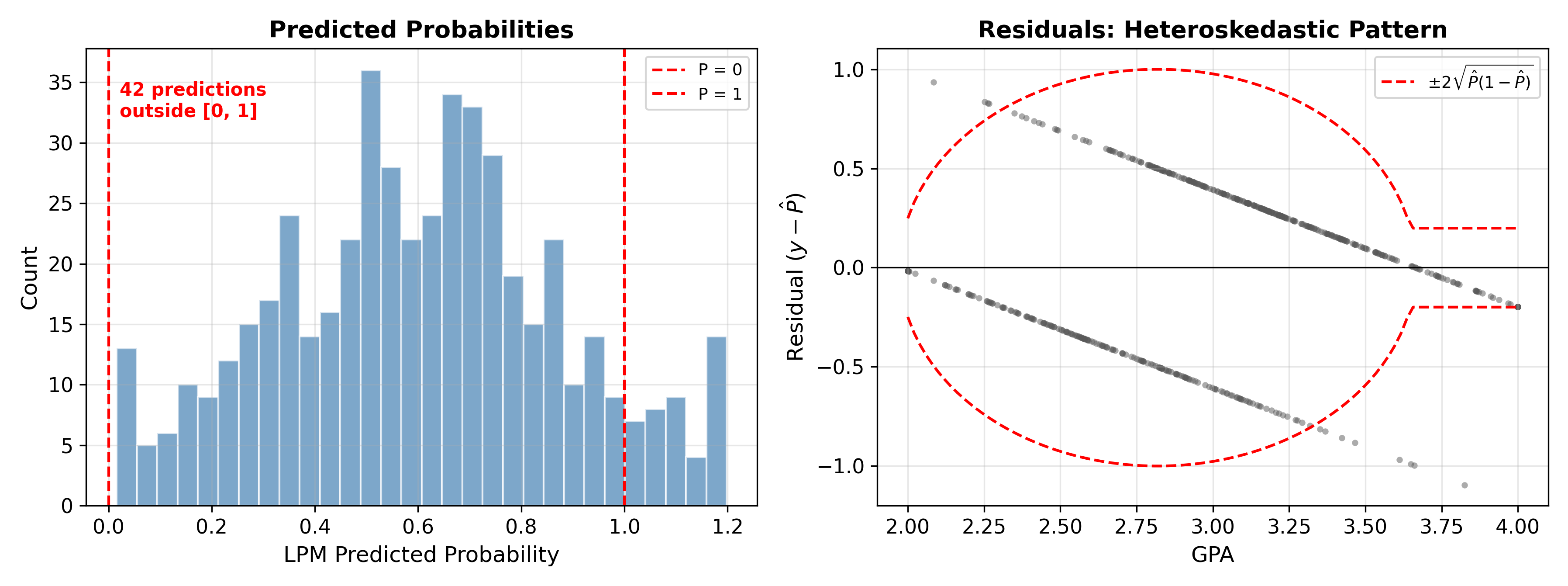
1. Impossible predictions. A linear function is unbounded. For sufficiently low GPA, the model predicts \(\hat{P} < 0\); for sufficiently high GPA, it predicts \(\hat{P} > 1\). Neither makes sense as a probability.
2. Constant marginal effects. The LPM assumes a one-unit increase in GPA always changes the admission probability by exactly \(\beta_1\), regardless of the starting point. But probabilities are bounded. Going from \(P = 0.01\) to \(P = 0.06\) is plausible; going from \(P = 0.95\) to \(P = 1.00\) with the same increment ignores the ceiling. The true marginal effect should be largest near \(P = 0.5\) and smallest near the boundaries.
3. Heteroskedastic errors. When \(y\) is binary, \(\text{Var}(y \mid x) = P(1 - P)\), which depends on \(x\). This violates homoskedasticity. OLS coefficient estimates remain unbiased, but standard errors are wrong without a robust correction.
Despite these problems, the LPM remains widely used in applied economics. Angrist and Pischke (2009) argue that it produces marginal effects close to logit/probit for most observations and avoids the computational overhead of nonlinear models.
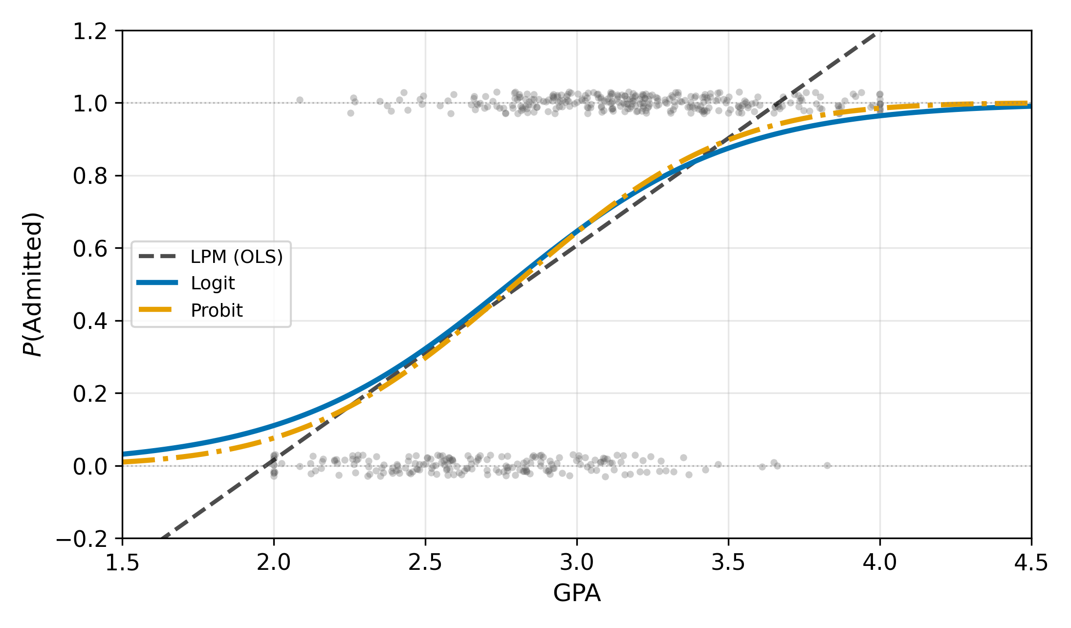
15.2 The S-Curve Solution
All three LPM problems stem from forcing a linear function onto a \([0, 1]\) outcome. The fix is to pass the linear index through a function that maps \((-\infty, +\infty)\) to \([0, 1]\). A CDF does exactly this.
15.2.1 The Latent Variable Framework
Many binary outcomes reflect an underlying continuous quantity we cannot observe. Whether a student is admitted depends on a continuous “admission index” that combines GPA, recommendations, essays, and luck. We call this unobserved quantity the latent variable \(y_i^*\):
\[ y_i^* = \beta_0 + \beta_1 \, \text{GPA}_i + \varepsilon_i \tag{15.2}\]
We observe only the binary outcome:
\[ y_i = \begin{cases} 1 & \text{if } y_i^* > 0 \\ 0 & \text{if } y_i^* \leq 0 \end{cases} \tag{15.3}\]
The probability of admission is then:
\[ P(y_i = 1 \mid x_i) = P(\varepsilon_i > -x_i'\beta) = 1 - F(-x_i'\beta) = F(x_i'\beta) \tag{15.4}\]
where \(F\) is the CDF of \(\varepsilon_i\) (the last equality holds when \(F\) is symmetric). The choice of \(F\) defines the model:
- Probit: \(F = \Phi\), the standard normal CDF. Assumes \(\varepsilon_i \sim N(0, 1)\).
- Logit: \(F = \Lambda\), the logistic CDF. Assumes \(\varepsilon_i\) follows a logistic distribution.
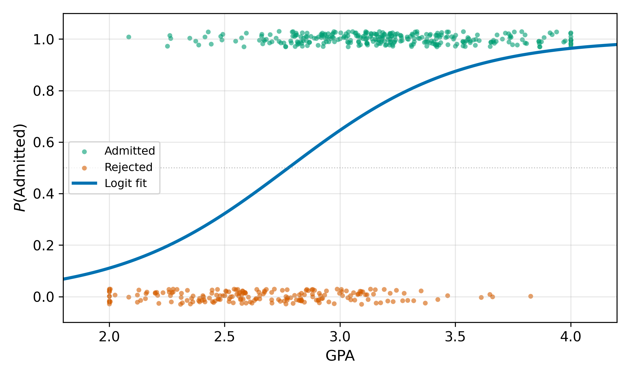
Both CDFs are S-shaped, increasing from 0 to 1. Both guarantee \(P \in [0, 1]\) for any value of \(x_i'\beta\). In the probit case, the marginal effect takes the form \(\partial P / \partial x = \phi(x'\beta) \cdot \beta_1\), where \(\phi\) is the standard normal PDF. The logit counterpart replaces \(\phi\) with \(\Lambda(1 - \Lambda)\). Both expressions say the same thing: the marginal effect is largest in the middle of the distribution and shrinks toward zero in the tails.
The logistic CDF has a closed form: \(\Lambda(z) = e^z / (1 + e^z)\). The normal CDF \(\Phi(z)\) does not, which is why probit requires numerical integration. In practice, software handles both seamlessly.
A CDF \(F(z)\) is defined as \(P(Z \leq z)\) for a random variable \(Z\). Probabilities are bounded between 0 and 1 by definition, so \(F(z) \in [0, 1]\) for all \(z\). As \(z \to -\infty\), \(F(z) \to 0\); as \(z \to +\infty\), \(F(z) \to 1\). The linear index \(x'\beta\) can take any real value, but the CDF compresses it into a valid probability.
15.3 Interpreting Logit Coefficients
In the LPM, \(\beta_1\) is the marginal effect: a one-unit increase in \(x\) changes the probability by \(\beta_1\). In logit, \(\beta_1\) is not the marginal effect. The logit model can be written as:
\[ \ln\left(\frac{p}{1-p}\right) = \beta_0 + \beta_1 x \tag{15.5}\]
The left side is the log-odds (or logit) of \(y = 1\). So \(\beta_1\) measures the change in log-odds for a one-unit increase in \(x\). Log-odds are not intuitive for most audiences \(\implies\) we need marginal effects.
15.3.1 Odds Ratios
Logit also has a convenient interpretation in terms of odds. The odds of \(y = 1\) are the ratio \(p / (1-p)\). From Equation 17.6:
\[ \frac{p}{1-p} = e^{\beta_0 + \beta_1 x} \tag{15.6}\]
A one-unit increase in \(x\) multiplies the odds by \(e^{\beta_1}\). If \(\beta_1 = 0.5\), then \(e^{0.5} \approx 1.65\), so each additional unit of \(x\) increases the odds by 65%. This multiplicative interpretation is why odds ratios are standard in epidemiology and clinical research.
15.3.2 Marginal Effects
Differentiating \(P = \Lambda(\beta_0 + \beta_1 x)\) with respect to \(x\):
\[ \frac{\partial P}{\partial x} = \beta_1 \cdot \Lambda(\beta_0 + \beta_1 x) \cdot \bigl[1 - \Lambda(\beta_0 + \beta_1 x)\bigr] \tag{15.7}\]
The marginal effect depends on where you are on the S-curve through the term \(\Lambda(\cdot)(1 - \Lambda(\cdot))\). This product is largest when \(\Lambda = 0.5\) (the midpoint of the curve) and shrinks toward zero at both extremes. \(\implies\) The same coefficient \(\beta_1\) produces different marginal effects for different observations.
Since the marginal effect varies, we need a summary measure. The average marginal effect (AME) evaluates the marginal effect at each observation’s actual \(x\) values and averages:
\[ \widehat{\text{AME}} = \frac{1}{N} \sum_{i=1}^{N} \hat{\beta}_1 \cdot \Lambda(\hat{\beta}_0 + \hat{\beta}_1 x_i) \cdot \bigl[1 - \Lambda(\hat{\beta}_0 + \hat{\beta}_1 x_i)\bigr] \tag{15.8}\]
An alternative is the marginal effect at the mean (MEM), which evaluates the marginal effect at \(x = \bar{x}\). The AME is generally preferred because it averages over the actual distribution of \(x\) rather than evaluating at a potentially unrepresentative point.
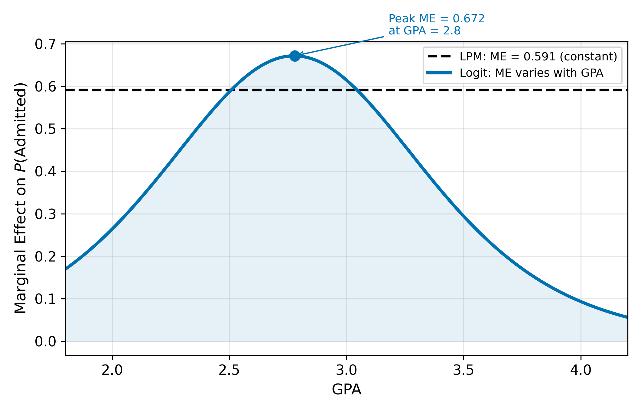
A useful approximation: at the point where \(P = 0.5\), the logit marginal effect is approximately \(\beta_1 / 4\). This “divide by four” rule gives a quick upper bound on the marginal effect without computing \(\Lambda\).
The marginal effect contains the factor \(P(1 - P)\). This is a quadratic in \(P\) that reaches its maximum at \(P = 0.5\), where \(P(1-P) = 0.25\). At \(P = 0.01\), the factor is \(0.01 \times 0.99 = 0.0099\); at \(P = 0.99\), it’s \(0.99 \times 0.01 = 0.0099\). Intuitively, when someone is almost certainly admitted (\(P \approx 1\)), a small increase in GPA barely changes anything. The room for movement is greatest when the outcome is most uncertain.
15.4 Logit vs. Probit
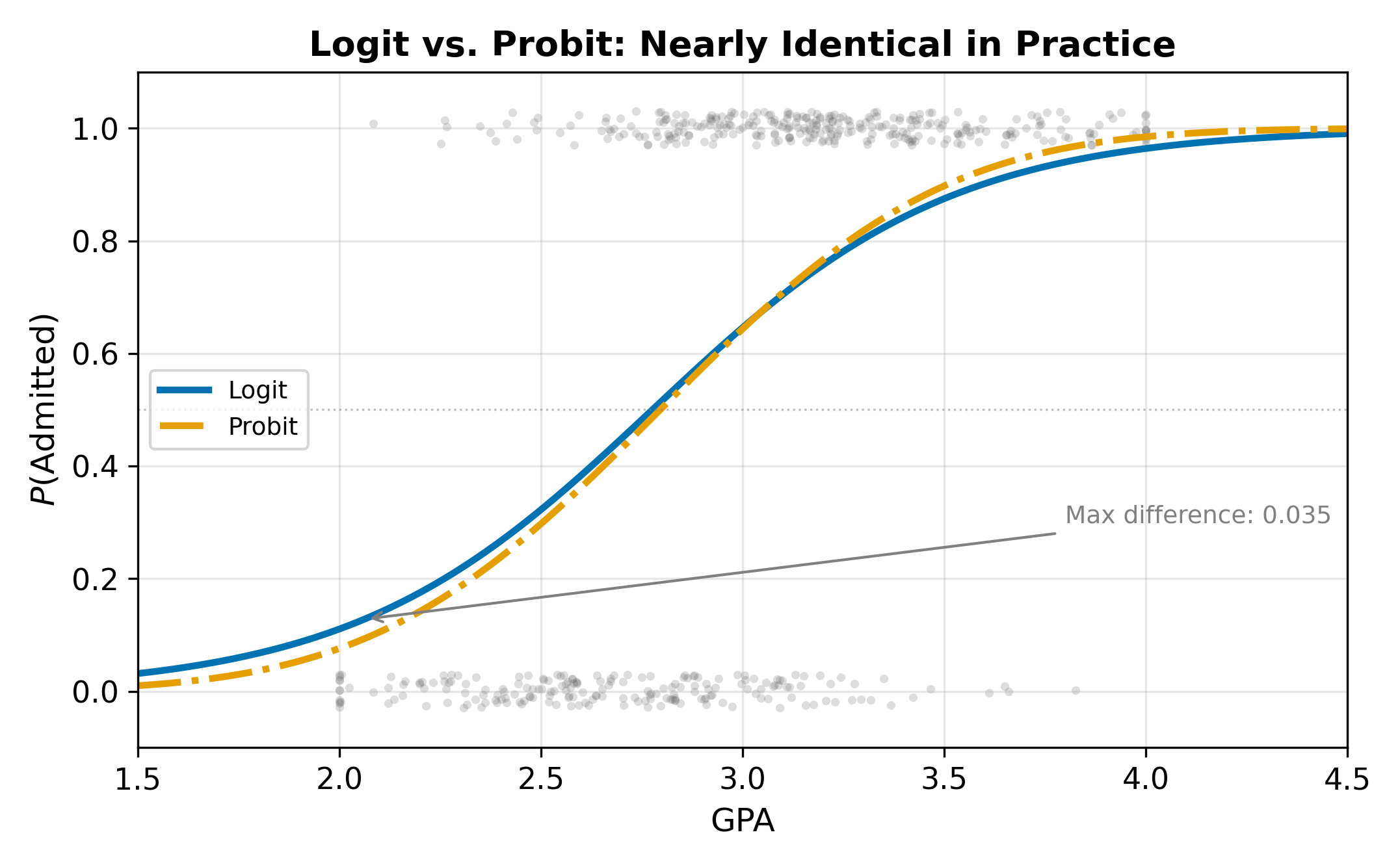
The logit and probit models use different CDFs but produce remarkably similar results in practice. The logistic distribution has slightly heavier tails than the normal, meaning logit assigns slightly more probability to extreme outcomes.
Because the logistic distribution has variance \(\pi^2/3 \approx 3.29\) while the standard normal has variance 1, the coefficients are on different scales:
\[ \hat{\beta}_{\text{Logit}} \approx 1.6 \, \hat{\beta}_{\text{Probit}} \tag{15.9}\]
This scaling means you cannot compare logit and probit coefficients directly. Compare predicted probabilities or marginal effects instead.
Logit is more common in epidemiology and machine learning (where odds ratios are standard currency). Probit is more common in economics (where the latent variable interpretation connects to structural models).
When to choose logit over probit:
- You want odds-ratio interpretations: \(e^{\beta_1}\) is the multiplicative change in odds for a one-unit increase in \(x\)
- You plan to extend to multinomial logit for unordered multi-category outcomes
- Your audience expects logit (clinical, ML contexts)
When to choose probit:
- The latent variable interpretation is needed for structural modeling
- You plan to extend to ordered probit or bivariate probit
- Your audience expects probit (most economics journals)
In either case, the predicted probabilities and AMEs will be nearly identical.
15.5 When Is the LPM Acceptable?
Despite its theoretical shortcomings, the LPM is sometimes the right tool:
When \(P\) is far from 0 and 1 for most observations. The S-curve and the line are nearly indistinguishable in the range \([0.2, 0.8]\). If your data lives in this region, the LPM’s linearity is inconsequential.
When you care about the AME, not tail probabilities. The LPM coefficient \(\beta_1\) is often close to the logit or probit AME. If you want a single summary of how \(x\) affects \(P\), the LPM delivers it without the machinery of MLE.
When you need instrumental variables or fixed effects. Nonlinear models combined with IV or FE raise incidental parameters problems and computational difficulties. The LPM, being linear, works seamlessly with these tools.
Speed and transparency. The LPM is OLS, so estimation is instant, convergence is guaranteed, and coefficients are directly interpretable.
\(\implies\) Use the LPM as a robustness check alongside logit or probit. If the AMEs agree, the choice of model is not driving your conclusions.
In practice, always report robust (heteroskedasticity-consistent) standard errors when using the LPM. The structural heteroskedasticity from \(\text{Var}(y \mid x) = P(1-P)\) makes conventional OLS standard errors unreliable.
15.6 Maximum Likelihood Estimation
We cannot estimate logit or probit with OLS because the model is nonlinear in \(\beta\). Instead, we use maximum likelihood estimation (MLE). The idea: find the parameter values that make the observed pattern of zeros and ones least surprising.
For each observation, the probability of seeing what we actually observed is:
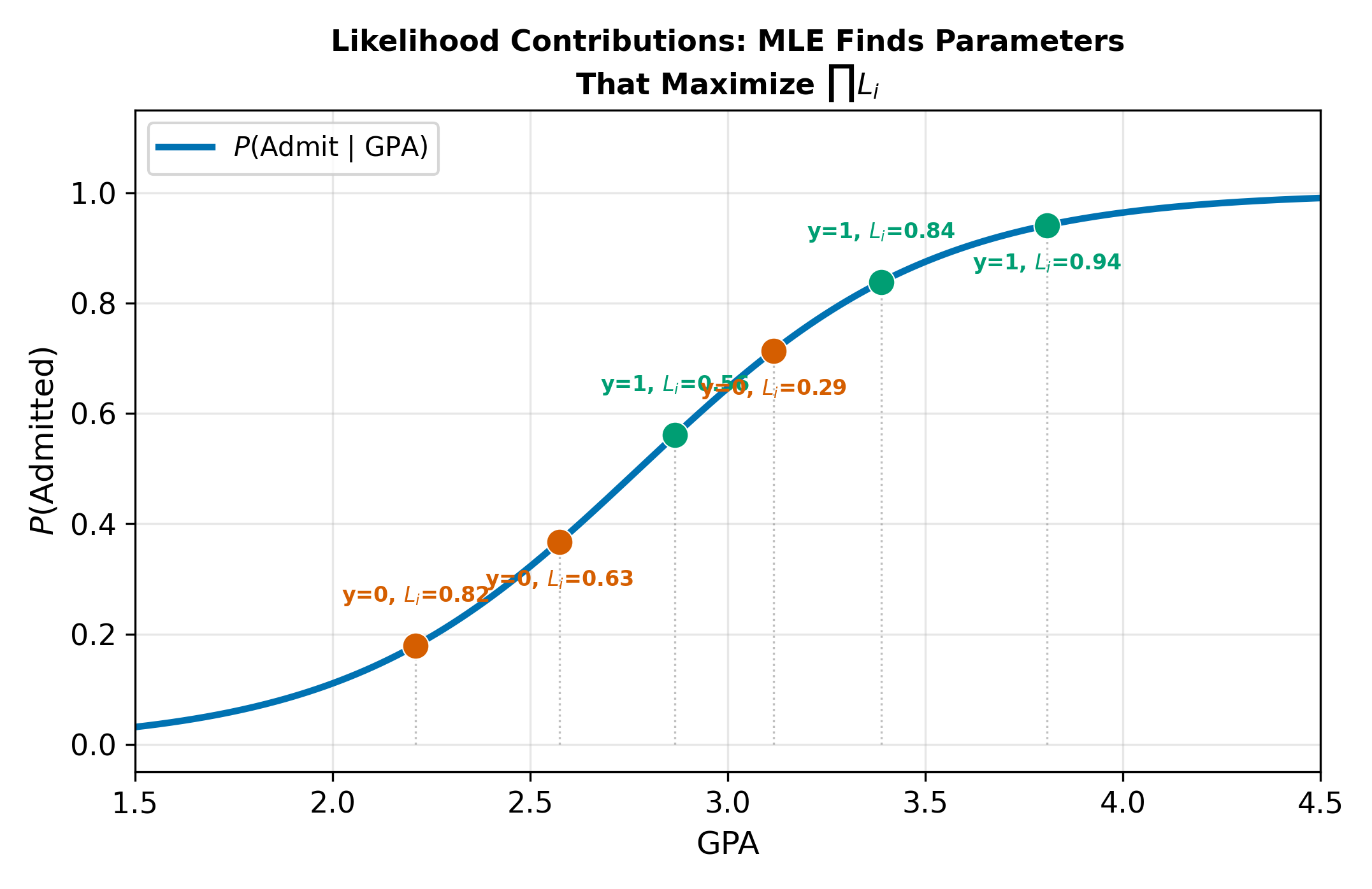
\[ L_i = P_i^{y_i}(1 - P_i)^{1-y_i} \tag{15.10}\]
When \(y_i = 1\), this equals \(P_i\); when \(y_i = 0\), it equals \(1 - P_i\). A good model assigns high \(P_i\) to observations where \(y_i = 1\) and low \(P_i\) where \(y_i = 0\).
The log-likelihood for the full sample sums across observations:
\[ \ell(\beta) = \sum_{i=1}^{N} \bigl[ y_i \ln P_i + (1-y_i) \ln(1-P_i) \bigr] \tag{15.11}\]
where \(P_i = F(\beta_0 + \beta_1 x_i)\). MLE finds the \(\beta\) that maximizes \(\ell(\beta)\). There is no closed-form solution; software uses iterative numerical optimization (Newton-Raphson or similar).
MLE properties are asymptotic: in large samples, MLE is consistent, asymptotically normal, and efficient (achieves the Cramer-Rao lower bound). In small samples, there are no finite-sample guarantees analogous to the Gauss-Markov theorem for OLS.
Think of it this way. If \(y_i = 1\) and the model assigns \(P_i = 0.95\), the contribution to the log-likelihood is \(\ln(0.95) = -0.05\), barely negative. If the model instead assigns \(P_i = 0.05\), the contribution is \(\ln(0.05) = -3.0\), dragging down the log-likelihood substantially. MLE picks the \(\beta\) values that make the data look as unsurprising as possible.
15.6.1 Hypothesis Testing
For individual coefficients, MLE uses the Wald test:
\[ z = \frac{\hat{\beta}_k}{\text{se}(\hat{\beta}_k)} \tag{15.12}\]
which is asymptotically standard normal under \(H_0: \beta_k = 0\). For joint restrictions (testing multiple coefficients simultaneously), the likelihood ratio (LR) test compares the unrestricted and restricted log-likelihoods:
\[ LR = 2(\ell_U - \ell_R) \sim \chi^2_{(J)} \tag{15.13}\]
where \(J\) is the number of restrictions. This is analogous to the F-test in OLS: if imposing the restrictions substantially reduces the fit (as measured by the log-likelihood), you reject.
15.6.2 Goodness of Fit
Standard \(R^2\) does not apply to MLE. The analog is McFadden’s pseudo-\(R^2\):
\[ \text{pseudo-}R^2 = 1 - \frac{\ln L_U}{\ln L_0} \tag{15.14}\]
where \(\ln L_U\) is the log-likelihood of the estimated model and \(\ln L_0\) is the log-likelihood of the intercept-only model. The scale differs from OLS \(R^2\); values above 0.2 typically indicate strong fit.
You can also report percent correctly predicted: classify each observation using a threshold (typically 0.5) and compare to actual outcomes. Neither measure is perfect, but together they give a reasonable sense of model performance. Be cautious with percent correctly predicted when the outcome is imbalanced. If 95% of applicants are admitted, a model that predicts “admitted” for everyone achieves 95% accuracy while being useless.
Ordered Choice Models extend the latent variable framework to outcomes with natural rankings (e.g., health satisfaction: low/medium/high). Return to the Qualitative and Limited DV hub for the full chapter map.