16 Ordered Choice Models
Modeling Ordinal Outcomes with Latent Variables and Cutpoints
Job satisfaction rated 1-5, credit ratings AAA to D, health status poor/fair/good/excellent, these outcomes are ordinal but not cardinal. Ordered choice models posit a latent continuous variable partitioned by estimated cutpoints. Covariates shift the distribution, changing the probability of each category.
This page assumes familiarity with the latent variable framework and maximum likelihood estimation from Qualitative and Limited Dependent Variable Models. The probit/logit background in Binary Choice Models is especially relevant since ordered models generalize binary ones to multiple ordered categories.
16.1 OLS on Ordinal Outcomes
A firm surveys employees on job satisfaction, rated 1 (Poor) through 5 (Excellent). Management wants to know whether wages, weekly hours, and supervisor support predict satisfaction. The natural first instinct is to code the categories as integers and run OLS:
\[ \text{Rating}_i = \beta_0 + \beta_1 \text{Wage}_i + \beta_2 \text{Hours}_i + \beta_3 \text{Support}_i + \varepsilon_i \tag{16.1}\]
This treats the categories as equally spaced on a cardinal scale. But there is no reason to believe that the gap between “Poor” (1) and “Fair” (2) is the same size as the gap between “Good” (4) and “Excellent” (5). OLS imposes that assumption by treating each one-unit increase as identical.
The difference between “Poor” (1) and “Fair” (2) need not equal the difference between “Good” (4) and “Excellent” (5). Ordinal data tells us the ranking but not the spacing.
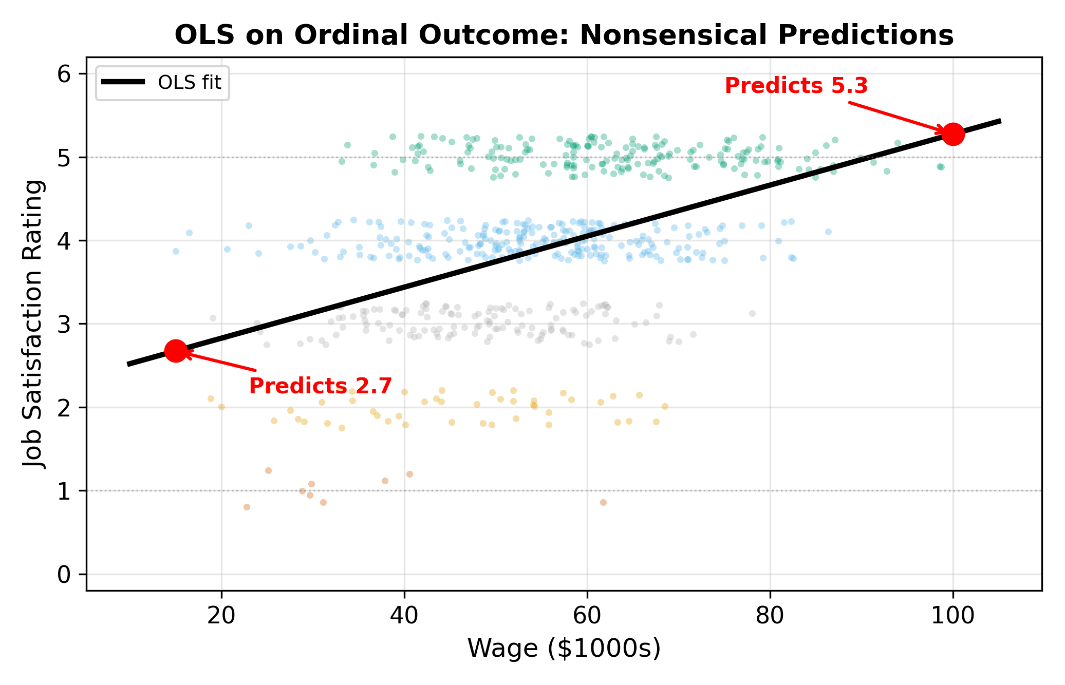
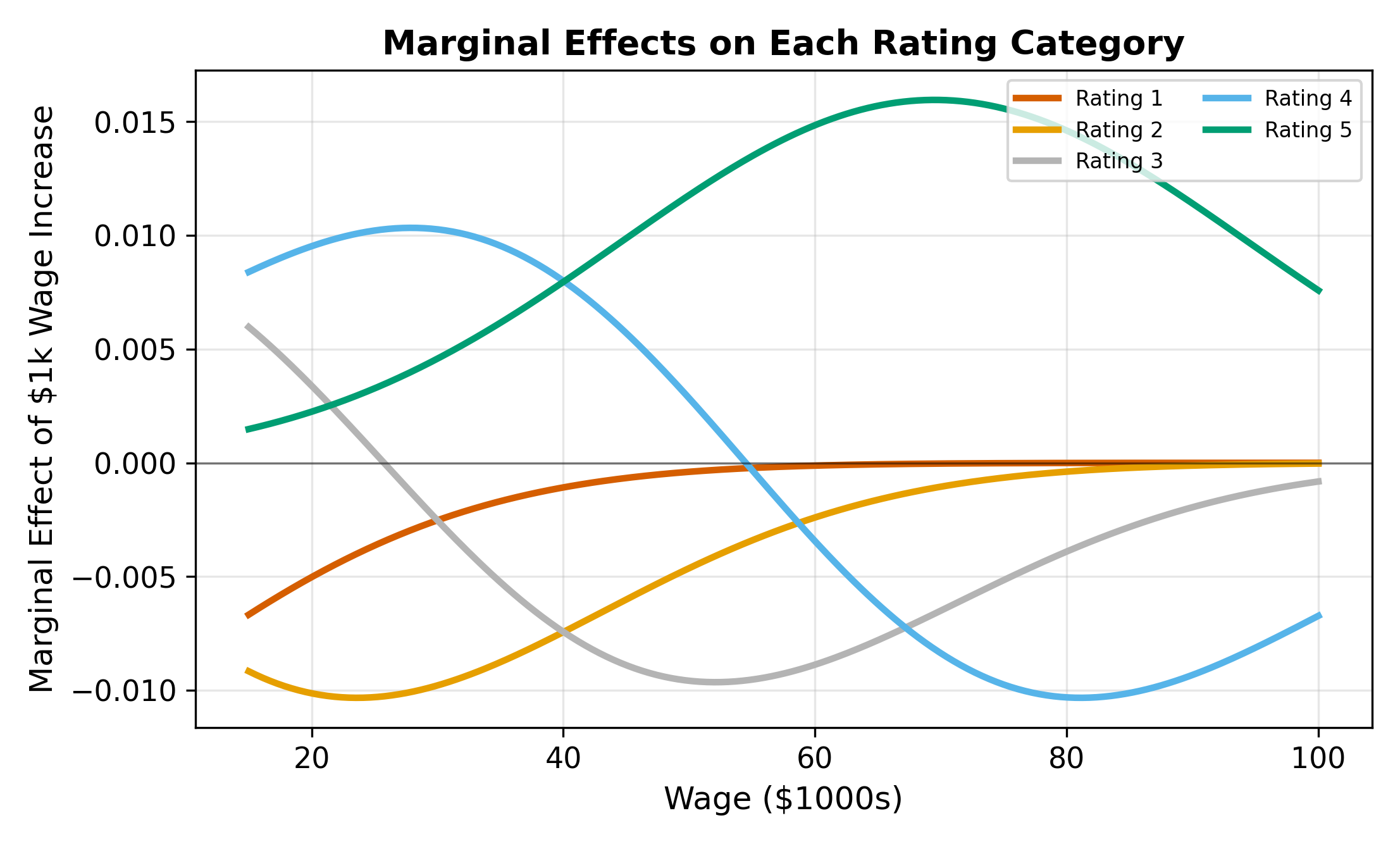
Beyond the spacing problem, OLS can predict values outside the valid range (e.g., \(\hat{y} = 0.3\) or \(\hat{y} = 5.7\)). It also forces constant marginal effects: a $1,000 wage increase always changes predicted satisfaction by the same amount, regardless of whether the worker is miserable or already content. These are the same issues that plague the linear probability model for binary outcomes, extended to the multi-category setting.
\(\implies\) We need a model that respects the ordinal nature of the dependent variable without imposing cardinal distances between categories.
16.2 The Latent Variable Model
The ordered probit/logit model assumes an unobserved (latent) continuous variable \(y_i^*\) drives the observed rating:
\[ y_i^* = \beta_1 \text{Wage}_i + \beta_2 \text{Hours}_i + \beta_3 \text{Support}_i + \varepsilon_i \tag{16.2}\]
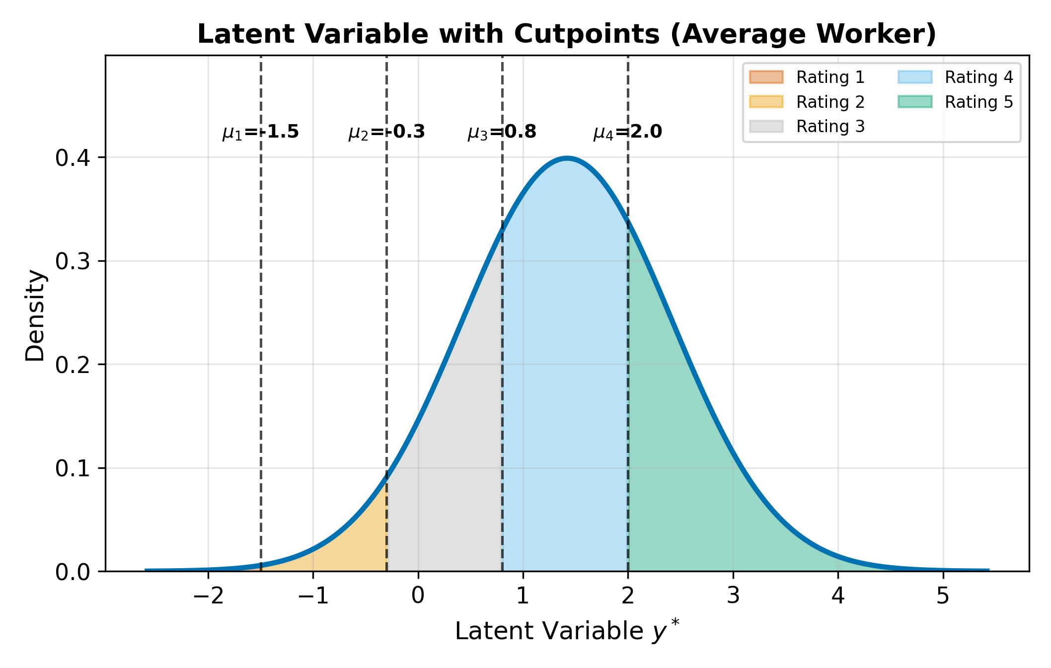
The latent variable represents the worker’s underlying satisfaction on a continuous scale. We never observe \(y_i^*\) directly. Instead, it gets mapped to the discrete rating through a set of cutpoints (also called thresholds) \(\mu_1 < \mu_2 < \mu_3 < \mu_4\):
\[ \text{Rating}_i = \begin{cases} 1 & \text{if } y_i^* \leq \mu_1 \\ 2 & \text{if } \mu_1 < y_i^* \leq \mu_2 \\ 3 & \text{if } \mu_2 < y_i^* \leq \mu_3 \\ 4 & \text{if } \mu_3 < y_i^* \leq \mu_4 \\ 5 & \text{if } y_i^* > \mu_4 \end{cases} \tag{16.3}\]
For \(J\) categories, there are \(J - 1\) cutpoints. The cutpoints are estimated alongside the \(\beta\) coefficients via maximum likelihood.
With \(J - 1\) cutpoints and no intercept, the model has \(J - 1 + K\) parameters, where \(K\) is the number of regressors. Binary probit is the special case \(J = 2\), one cutpoint.
The intercept and the cutpoints are not separately identified. If you added an intercept \(\beta_0\) to Equation 16.2, you could always shift \(\beta_0\) up by some constant \(c\) and shift every cutpoint \(\mu_j\) up by the same \(c\) without changing any of the category probabilities. To resolve this, the convention is to drop the intercept and let the cutpoints absorb the location of the distribution.
This is the same identification issue that forces us to normalize \(\sigma = 1\) in binary probit: the latent scale has no natural units, so we need to fix enough parameters to pin it down.
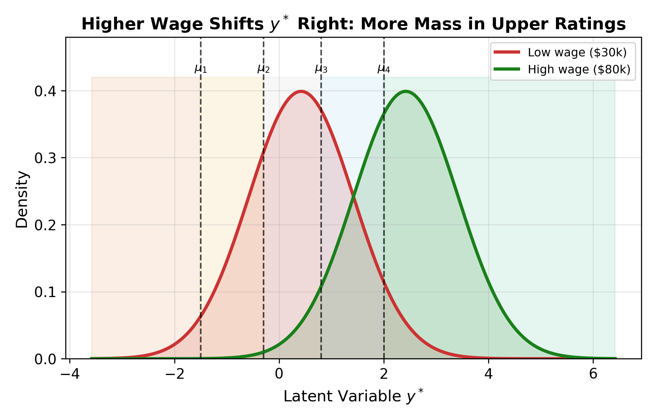
The figure above shows the core mechanism. The cutpoints stay fixed in place. When a covariate changes (e.g., wages increase), the entire latent distribution shifts. A rightward shift (positive \(\beta\)) pushes more probability mass past the upper cutpoints, raising the likelihood of higher categories.
16.3 The Probability Formula
The probability of observing category \(j\) for individual \(i\) comes directly from the latent variable model. Since \(\text{Rating}_i = j\) whenever \(\mu_{j-1} < y_i^* \leq \mu_j\):
\[ P(\text{Rating}_i = j) = F(\mu_j - X_i\beta) - F(\mu_{j-1} - X_i\beta) \tag{16.4}\]
where \(F\) is the CDF of \(\varepsilon\), \(X_i\beta = \beta_1 \text{Wage}_i + \beta_2 \text{Hours}_i + \beta_3 \text{Support}_i\), and we set \(\mu_0 = -\infty\) and \(\mu_J = +\infty\) for the boundary categories.
- Ordered probit: \(F = \Phi\) (standard normal CDF)
- Ordered logit: \(F = \Lambda\) (logistic CDF)
The cutpoints \(\mu_j\) are estimated alongside the \(\beta\)’s via MLE. The log-likelihood sums \(\ln P(\text{Rating}_i = j_i)\) over all observations, where \(j_i\) is the category actually observed for person \(i\).
16.3.1 Numeric Example
Suppose the estimated model yields \(\hat{\mu}_1 = -1.8\), \(\hat{\mu}_2 = -0.5\), \(\hat{\mu}_3 = 0.6\), \(\hat{\mu}_4 = 1.9\), and for a particular worker \(X_i\hat{\beta} = 0.4\). Using ordered probit (\(F = \Phi\)):
\[ \begin{aligned} P(\text{Rating} = 1) &= \Phi(-1.8 - 0.4) = \Phi(-2.2) = 0.014 \\ P(\text{Rating} = 2) &= \Phi(-0.5 - 0.4) - \Phi(-1.8 - 0.4) = \Phi(-0.9) - \Phi(-2.2) = 0.170 \\ P(\text{Rating} = 3) &= \Phi(0.6 - 0.4) - \Phi(-0.5 - 0.4) = \Phi(0.2) - \Phi(-0.9) = 0.395 \\ P(\text{Rating} = 4) &= \Phi(1.9 - 0.4) - \Phi(0.6 - 0.4) = \Phi(1.5) - \Phi(0.2) = 0.348 \\ P(\text{Rating} = 5) &= 1 - \Phi(1.9 - 0.4) = 1 - \Phi(1.5) = 0.067 \end{aligned} \tag{16.5}\]
The five probabilities sum to 1. This worker is most likely to report a rating of 3 or 4.
16.4 Interpretation and Marginal Effects
16.4.1 Coefficients Give Direction Only
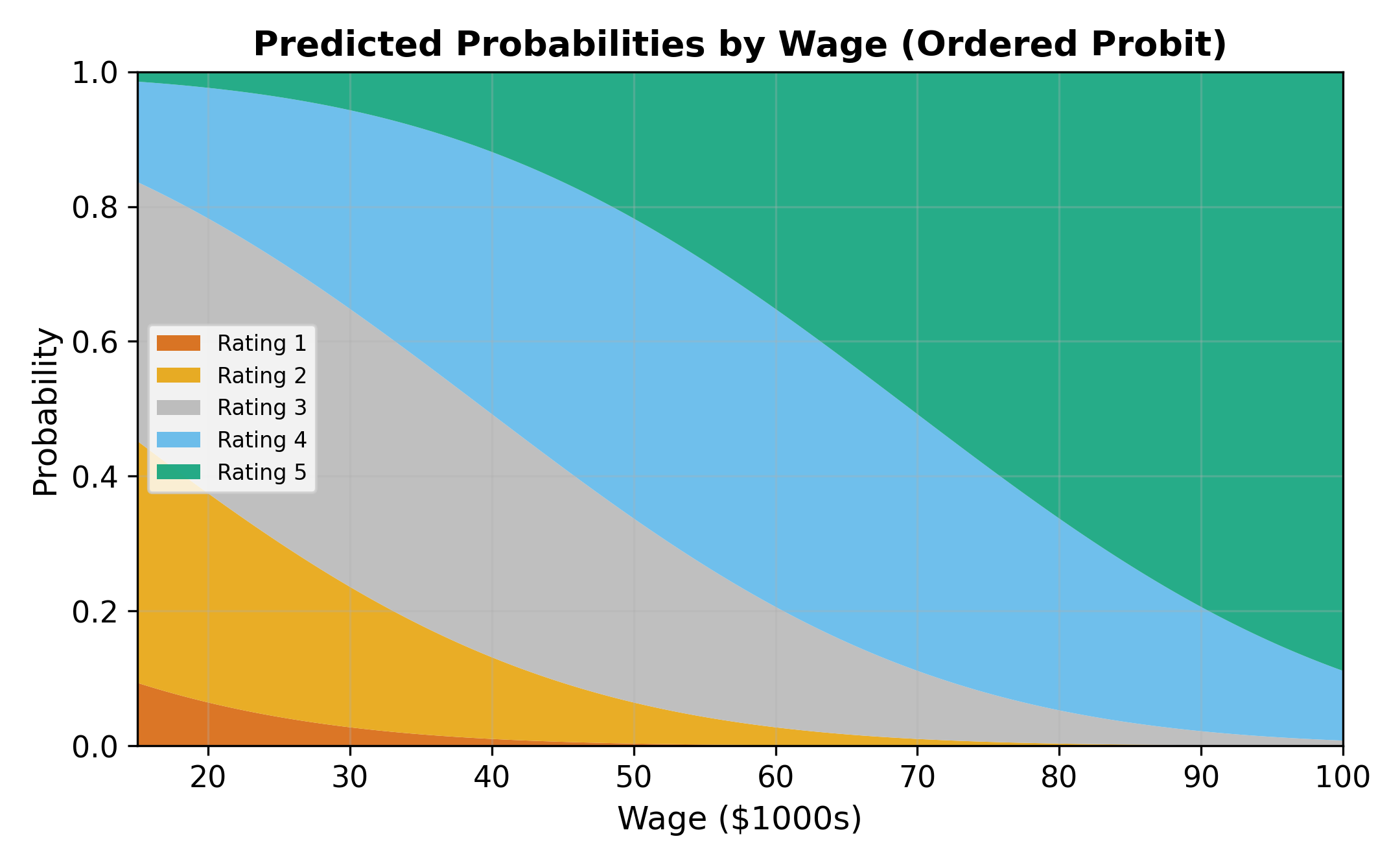
Unlike OLS, the \(\beta\) coefficients in ordered probit/logit do not directly tell you the magnitude of the effect on any particular category. A positive \(\beta_k\) means that increasing \(x_k\) shifts the latent distribution to the right, which:
- Always increases \(P(\text{highest category})\)
- Always decreases \(P(\text{lowest category})\)
- Has an ambiguous effect on middle categories
\(\implies\) Always compute marginal effects. Never interpret raw ordered model coefficients as though they were OLS slopes.
16.4.2 The Marginal Effect Formula
For a continuous covariate \(x_k\):
\[ \frac{\partial P(\text{Rating} = j)}{\partial x_k} = \left[ f(\mu_{j-1} - X\beta) - f(\mu_j - X\beta) \right] \cdot \beta_k \tag{16.6}\]
where \(f\) is the PDF corresponding to \(F\) (standard normal density \(\phi\) for probit, logistic density \(\lambda\) for logit).
For the extreme categories, the marginal effect simplifies because one of the boundary terms vanishes (\(f(-\infty) = 0\) or \(f(+\infty) = 0\)):
\[ \frac{\partial P(\text{Rating} = 1)}{\partial x_k} = -f(\mu_1 - X\beta) \cdot \beta_k \tag{16.7}\]
\[ \frac{\partial P(\text{Rating} = J)}{\partial x_k} = f(\mu_{J-1} - X\beta) \cdot \beta_k \tag{16.8}\]
For extreme categories, the sign of the marginal effect always matches (highest) or opposes (lowest) the sign of \(\beta_k\). For middle categories, the sign depends on the balance between the two density terms, which varies with \(X\beta\).
These have unambiguous signs: if \(\beta_k > 0\), the probability of the highest category increases and the probability of the lowest category decreases.
For middle categories, the sign of the marginal effect depends on the bracketed term \([f(\mu_{j-1} - X\beta) - f(\mu_j - X\beta)]\). This difference can be positive or negative depending on where the individual’s \(X\beta\) falls relative to the cutpoints.
16.4.3 Marginal Effects Sum to Zero
Across all \(J\) categories, the marginal effects must sum to zero:
\[ \sum_{j=1}^{J} \frac{\partial P(\text{Rating} = j)}{\partial x_k} = 0 \tag{16.9}\]
If an increase in \(x_k\) pushes probability mass toward higher categories, that mass must come from somewhere. The total probability is always 1, so gains in some categories are offset by losses in others.
Consider a worker whose \(X\beta\) places them right at cutpoint \(\mu_3\). A small increase in wages shifts the latent distribution rightward. This pulls probability mass from both sides of \(\mu_3\). Mass from category 3 shifts into category 4, and mass from category 2 shifts into category 3. If the outflow (3 to 4) exceeds the inflow (2 to 3), the net effect on \(P(\text{Rating} = 3)\) is negative, despite \(\beta > 0\).
The sign of the middle-category effect depends on the shape of the density at the two adjacent cutpoints. When the density is higher at the upper cutpoint than the lower one, the outflow dominates.
16.4.4 Binary Covariates: Discrete Differences
For a binary variable (e.g., a training program indicator), compute the discrete change rather than the derivative. Calculate predicted probabilities with the dummy set to 0 and then to 1, holding other covariates at their means or observed values:
\[ \Delta P(\text{Rating} = j) = P(\text{Rating} = j \mid D = 1) - P(\text{Rating} = j \mid D = 0) \]
16.5 The Parallel Regressions Assumption
Ordered probit and logit impose a restriction called the parallel regressions assumption (also known as the proportional odds assumption in the logit case): the same coefficient vector \(\beta\) applies at every cutpoint. Only the cutpoints \(\mu_j\) differ across category boundaries.
This means that a $1,000 wage increase shifts the latent distribution by the same amount regardless of whether we are looking at the boundary between “Poor” and “Fair” or the boundary between “Good” and “Excellent.” The effect of each covariate is the same across all thresholds.
Testing the parallel regressions assumption: estimate a series of binary models (collapsing categories at each cutpoint) and compare coefficients. If they differ substantially, the assumption may not hold. The Brant test formalizes this comparison.
When this assumption fails, the model is misspecified. Consider:
- Generalized ordered logit: allows \(\beta\) to differ across cutpoints
- Multinomial logit: drops the ordering assumption entirely (but discards ordering information)
In practice, the parallel regressions assumption is a strong restriction. Always think about whether it is reasonable for the specific application. If the factors driving someone from “Poor” to “Fair” are fundamentally different from those driving someone from “Good” to “Excellent,” ordered probit/logit may not be appropriate.
16.6 Ordered vs. Multinomial
Both ordered and multinomial models handle dependent variables with more than two categories. The choice depends on whether the categories have a natural ranking.
| Feature | Ordered Probit/Logit | Multinomial Logit |
|---|---|---|
| Category structure | Natural ordering (low to high) | No ordering (unranked) |
| Number of \(\beta\) vectors | 1 (shared across cutpoints) | \(J - 1\) (one per non-base category) |
| Parsimony | More parsimonious | More flexible |
| Uses ordering info | Yes | No (ignores ranking) |
| Example | Satisfaction ratings, credit grades | Transport mode, brand choice |
Decision rule:
- If categories have a clear ranking (satisfaction: low \(<\) medium \(<\) high), use ordered probit/logit.
- If categories are unranked (transport: car, bus, train), use multinomial logit.
- If categories are ranked but the parallel regressions assumption fails, consider generalized ordered logit or, as a fallback, multinomial logit.
\(\implies\) Using multinomial logit on ordered data wastes information. Using ordered models on unordered data imposes a false ranking. Match the model to the data structure.
Multinomial Logit covers unordered categorical outcomes, where the IIA assumption and alternative-specific covariates become central. See also the hub page for the full limited dependent variable roadmap.