Chapter 16: Discussion Problems

Qualitative and Limited Dependent Variables

Qualitative and Limited DV

Discussion Problems

Author

Jake Anderson

Published

March 3, 2026

Modified

March 4, 2026

Prerequisites

These problems accompany Qualitative and Limited Dependent Variables and its sub-pages on Binary Choice, Ordered Choice, and Multinomial Logit. Read those first for the theory behind these exercises.

Discussion Problems

Question 16.18

Mortgage lenders are interested in determining borrower and loan characteristics that may lead to delinquency or foreclosure. In the data file lasvegas are 1000 observations on mortgages for single family homes in Las Vegas, Nevada during 2008. The variable of interest is $DELINQUENT$, an indicator variable = 1 if the borrower missed at least three payments (90+ days late), but 0 otherwise. Explanatory variables are $LVR$ = the ratio of the loan amount to the value of the property; $REF$ = 1 if the purpose of the loan was a “refinance” and = 0 if the loan was for a purchase; $INSUR$ = 1 if the mortgage carries mortgage insurance, 0 otherwise; $RATE$ = initial interest rate of the mortgage; $AMOUNT$ = dollar value of mortgage (in $\$100,000$); $CREDIT$ = credit score; $TERM$ = number of years between disbursement of the loan and the date it is expected to be fully repaid, $ARM$ = 1 if the mortgage has an adjustable rate, and = 0 if the mortgage has a fixed rate.

Show code

lasvegas <- read.csv("data/lasvegas.csv")

Variable Definitions

Dependent variable:

$DELINQUENT$: equals 1 if the borrower is 90+ days late on their mortgage

Continuous regressors:

$LVR$: loan-to-value ratio (%). How much of the home’s value is financed. Higher LVR $\implies$ less equity cushion
$RATE$: initial interest rate (%). Higher rate $\implies$ larger monthly payments
$CREDIT$: credit score (300–850). Summarizes past repayment behavior
$AMOUNT$: loan amount in $100K units (e.g., 2.5 = $250K)
$TERM$: loan term in years (e.g., 15 or 30). Longer term $\implies$ smaller payments but slower equity buildup

Binary regressors:

$REF$: equals 1 if refinance (vs. new purchase). May signal financial stress
$INSUR$: equals 1 if mortgage insurance (typically required when $LVR > 80$). Protects the lender, not the borrower
$ARM$: equals 1 if adjustable-rate mortgage. Carries payment shock risk when rates rise

Part A

Estimate the linear probability model explaining $DELINQUENT$ as a function of the remaining variables. Use White heteroskedasticity robust standard errors. Are the signs of the estimated coefficients reasonable?

Solution

Show code

vegas.lpm <- lm(DELINQUENT ~ ., data = lasvegas)
coeftest(vegas.lpm, vcov. = vcovHC(vegas.lpm, type = "HC1"))


t test of coefficients:

              Estimate Std. Error t value Pr(>|t|)    
(Intercept)  0.6884913  0.2285064   3.013 0.002652 ** 
LVR          0.0016239  0.0006752   2.405 0.016360 *  
REF         -0.0593237  0.0240256  -2.469 0.013710 *  
INSUR       -0.4815849  0.0303694 -15.858  < 2e-16 ***
RATE         0.0343761  0.0098194   3.501 0.000484 ***
AMOUNT       0.0237680  0.0144509   1.645 0.100340    
CREDIT      -0.0004419  0.0002073  -2.132 0.033262 *  
TERM        -0.0126195  0.0035560  -3.549 0.000405 ***
ARM          0.1283239  0.0276932   4.634 4.07e-06 ***
---
Signif. codes:  0 '***' 0.001 '**' 0.01 '*' 0.05 '.' 0.1 ' ' 1

The signs on the estimated coefficients are reasonable. As the loan to home value ratio increases, the rate of delinquency increases. Refinanced loans are less likely to be delinquent, which is reasonable as banks would likely refinance individuals with a history of timely payments. The estimated coefficient indicates that mortgages that carry insurance (often for small down payments), are less likely to be delinquent. As interest rates increase, it is more likely that the loan becomes delinquent. As the credit score increases, it becomes less likely for the loan to be delinquent. As the term of the loan increases, it is less likely to become delinquent. Adjustable rate mortgages are more likely to become delinquent.

Part B

Use logit to estimate the model in (a). Are the signs and significance of the estimated coefficients the same as for the linear probability model?

Solution

Show code

vegas.logit <- glm(DELINQUENT ~ ., data = lasvegas, family = binomial(link = "logit"))
summary(vegas.logit)


Call:
glm(formula = DELINQUENT ~ ., family = binomial(link = "logit"), 
    data = lasvegas)

Coefficients:
            Estimate Std. Error z value Pr(>|z|)    
(Intercept)  1.66530    1.99216    0.84  0.40319    
LVR          0.01352    0.00820    1.65  0.09916 .  
REF         -0.52506    0.23049   -2.28  0.02273 *  
INSUR       -3.12211    0.21691  -14.39  < 2e-16 ***
RATE         0.30866    0.08277    3.73  0.00019 ***
AMOUNT       0.21761    0.11377    1.91  0.05579 .  
CREDIT      -0.00356    0.00193   -1.84  0.06523 .  
TERM        -0.13304    0.03460   -3.85  0.00012 ***
ARM          1.40565    0.37136    3.79  0.00015 ***
---
Signif. codes:  0 '***' 0.001 '**' 0.01 '*' 0.05 '.' 0.1 ' ' 1

(Dispersion parameter for binomial family taken to be 1)

    Null deviance: 998.03  on 999  degrees of freedom
Residual deviance: 666.29  on 991  degrees of freedom
AIC: 684.3

Number of Fisher Scoring iterations: 5

The estimated coefficients all carry the same signs, however the coefficient on loan amount is now significant.

Part C

Compute the predicted value of $DELINQUENT$ for the 500th and 1000th observations using both the linear probability model and the logit model. Interpret the values.

Solution

Show code

predict(vegas.lpm, lasvegas[c(500, 1000), ])

     500     1000 
0.182783 0.578530

Show code

predict(vegas.logit, lasvegas[c(500, 1000), ], type = "response")

     500     1000 
0.133585 0.626553

For the 500th observation, the LPM predicts the individual had an $18.3\%$ probability of delinquency, while the logit model predicted a $13.4\%$ probability of delinquency. For the 1000th observation, the LPM predicts the individual had an $57.9\%$ probability of delinquency, while the logit model predicted a $62.7\%$ probability of delinquency.

Part D/E

Construct a histogram of $CREDIT$. Using both models, calculate the probability of delinquency for $CREDIT$ = 500, 600, and 700 for a loan of $\$250,000$. For the other variables, let the $LVR$ be $80\%$, the initial interest rate be $8\%$, all indicator variables taking the value 0, and $TERM = 30$. Discuss the similarities and differences among the predicted probabilities from the two models. Using both linear probability and logit models, compute the marginal effect of $CREDIT$ on the probability of delinquency.

Solution

Show code

hist(lasvegas$CREDIT, main = "", xlab = "Credit score", breaks = 14)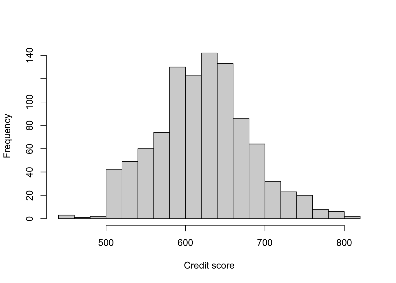

Show code

## Predictions
characteristics <- data.frame(CREDIT = c(500, 600, 700),
                               AMOUNT = 2.5,
                               LVR    = 80,
                               RATE   = 8,
                               TERM   = 30,
                               INSUR  = 0,
                               REF    = 0,
                               ARM    = 0)
predict(vegas.lpm, characteristics)

       1        2        3 
0.553296 0.509106 0.464917

Show code

predict(vegas.logit, characteristics, type = "response")

       1        2        3 
0.496703 0.408631 0.326058

Given these loan characteristics, the logit model predicts lower rates of default across all credit scores. One interesting thing to note is the change in marginal effect. In the LPM, moving from a credit score of 500 to a credit score of 600 reduces default probability by the same amount as moving from a credit score of 600 to a credit score of 700. In both cases, the probability of default decreases by $4.42$ percentage points. In comparison, the logit model has different marginal effects. Moving from 500 to 600 reduces the probability of default by $8.81$ percentage points, while moving from 600 to 700 reduces the probability of default by $8.26$ percentage points.

Part F

Construct a histogram of LVR. Using both the LPM and logit models, calculate the probability of delinquency for $LVR = 20$ and $LVR = 80$, with $CREDIT = 600$ and other variables set as they are in (d). Compare and contrast the results.

Solution

Show code

hist(lasvegas$LVR, main = "", xlab = "Loan-to-value ratio", breaks = 14)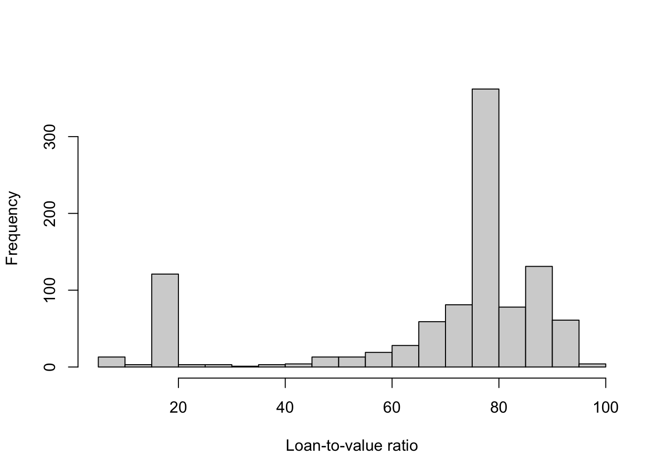

Show code

## Predictions
characteristics <- data.frame(CREDIT = 600,
                               AMOUNT = 2.5,
                               LVR    = c(20, 80),
                               RATE   = 8,
                               TERM   = 30,
                               INSUR  = 0,
                               REF    = 0,
                               ARM    = 0)
predict(vegas.lpm, characteristics)

       1        2 
0.411675 0.509106

Show code

predict(vegas.logit, characteristics, type = "response")

       1        2 
0.234909 0.408631

The logit model makes much lower predictions for delinquency probabilities than the linear model, and has a much larger marginal effect when moving from an $LVR$ of 20% to an $LVR$ of 80%.

Part G

Compare the percentage of correct predictions from the linear probability model and the logit model using a predicted probability of $0.5$ as the threshold.

Solution

Show code

pred.lpm <- as.numeric(predict(vegas.lpm) > 0.5)
pred.logit <- as.numeric(predict(vegas.logit, type = "response") > 0.5)

The linear probability model correctly predicts 858 delinquency outcomes, while the logit model correctly predicts 854.

Part H

As a loan officer, you wish to provide loans to customers who repay on schedule and are not delinquent. Suppose you have available to you the first 500 observations in the data on which to base your loan decisions on the second 500 applications (501–1,000). Is using the logit model with a threshold of $0.5$ for the predicted probability the best decision rule for deciding on loan applications? If not, what is a better rule?

Solution

Show code

training.logit <- glm(DELINQUENT ~ ., data = lasvegas[1:500, ],
                       family = binomial(link = "logit"))
test.pred <- predict(training.logit, newdata = lasvegas[501:1000, ],
                      type = "response")
true.pred <- numeric(100)
for (i in 1:100) {
  true.pred[i] <- sum(as.numeric(test.pred > i / 100) == lasvegas[501:1000, "DELINQUENT"])
}

The threshold of $0.5$ correctly predicts 440 applications in the test sample, while the optimal threshold of $0.49$ accurately predicts 442 applications. However, this method does not account for the differences between a false positive vs. false negative. It is likely that loan officers would rather err on the side of caution and pick a cutoff that minimizes the likelihood of clearing a loan that turns delinquent, instead of a policy that incorrectly assumes someone will make delinquent payments.

Question 16.23

How well do age, education, and other personal characteristics predict our assessment of our health status? Use the data file rwm88 to answer the following.

Show code

rwm88 <- read.csv("data/rwm88.csv")

Part A

Tabulate the variable $HSAT3$, which is a self-rating of health satisfaction, with $1$ being the lowest and $3$ being the highest. What percent of the sample assess their health status as $HSAT3 = 1, 2,$ or $3$?

Solution

Show code

table(rwm88$hsat3)


   1    2    3 
1777 1792  914

Part B

Estimate an ordered probit model predicting $HSAT3$ using $AGE$, $AGE^{2}$, $EDUC2$ = years of education, and $WORKING$ = 1 if employed. Which variables have coefficients that are statistically significant at the $5\%$ level?

Solution

Show code

hsac.probit <- polr(factor(hsat3) ~ age + I(age^2) + educ2 + working,
                    data = rwm88, method = "probit")
summary(hsac.probit)

Call:
polr(formula = factor(hsat3) ~ age + I(age^2) + educ2 + working, 
    data = rwm88, method = "probit")

Coefficients:
             Value Std. Error t value
age      -0.055709  0.0050842  -10.96
I(age^2)  0.000408  0.0000725    5.62
educ2     0.047848  0.0073468    6.51
working   0.091071  0.0382128    2.38

Intercepts:
    Value     Std. Error t value  
1|2    -1.253     0.001  -1124.772
2|3    -0.119     0.023     -5.175

Residual Deviance: 9205.95 
AIC: 9217.95

All the coefficients are statistically significant at the 5% level.

Part C

Estimate the marginal impact of age on the probabilities of health satisfactions $HSAT3 = 1, 2,$ or $3$ for someone age $40$, with 16 years of education, and who is working.

Solution

Let \[\begin{align*} \hat{y}_{1} &= \hat\mu_{1} - \hat\beta_{1}AGE - \hat\beta_{2}AGE^{2} - \hat\beta_{3}EDUC2 - \hat\beta_{4}WORKING\\ \hat{y}_{2} &= \hat\mu_{2} - \hat\beta_{1}AGE - \hat\beta_{2}AGE^{2} - \hat\beta_{3}EDUC2 - \hat\beta_{4}WORKING \end{align*}\] The marginal effects are calculated with the following formula:

\[\begin{align*} \frac{\partial P(HSAT3 = 3|X)}{\partial AGE} &= \phi(\hat{y_{2}})\times(\beta_{1} + 2\beta_{2}AGE)\\ \frac{\partial P(HSAT3 = 2|X)}{\partial AGE} &= \left[\phi(\hat{y_{1}}) - \phi(\hat{y_{2}})\right]\times(\beta_{1} + 2\beta_{2}AGE)\\ \frac{\partial P(HSAT3 = 1|X)}{\partial AGE} &= - \phi(\hat{y_{1}})\times(\beta_{1} + 2\beta_{2}AGE)\\ \end{align*}\]

Show code

## Pull coefficients and X variables to plug into the predictions
coef <- as.numeric(hsac.probit$coefficients)
cutoffs <- as.numeric(hsac.probit$zeta)
characteristics <- c(40, 40^2, 16, 1)

## Calculate the latent values in the probit model
y1 <- cutoffs[1] - sum(coef * characteristics)
y2 <- cutoffs[2] - sum(coef * characteristics)

## Calculate the marginal effects
me3 <- dnorm(y2) * (coef[1] + 2 * coef[2] * characteristics[1])
me2 <- (dnorm(y1) - dnorm(y2)) * (coef[1] + 2 * coef[2] * characteristics[1])
me1 <- -dnorm(y1) * (coef[1] + 2 * coef[2] * characteristics[1])

\[\begin{align*} \frac{\partial P(HSAT3 = 3|X)}{\partial AGE} &= -0.770\%\\ \frac{\partial P(HSAT3 = 2|X)}{\partial AGE} &= -0.030\%\\ \frac{\partial P(HSAT3 = 1|X)}{\partial AGE} &= 0.800\%\\ \end{align*}\]

(Note that the marginal effects add up to zero!)

Part D

Estimate the marginal impact of age on the probabilities of health satisfaction $HSAT3 = 1, 2,$ or $3$ for someone age $70$, with 16 years of education, and who is working.

Solution

Show code

## Pull coefficients and X variables to plug into the predictions
coef <- as.numeric(hsac.probit$coefficients)
cutoffs <- as.numeric(hsac.probit$zeta)
characteristics <- c(70, 70^2, 16, 1)

## Calculate the latent values in the probit model
y1 <- cutoffs[1] - sum(coef * characteristics)
y2 <- cutoffs[2] - sum(coef * characteristics)

## Calculate the marginal effects
me3 <- dnorm(y2) * (coef[1] + 2 * coef[2] * characteristics[1])
me2 <- (dnorm(y1) - dnorm(y2)) * (coef[1] + 2 * coef[2] * characteristics[1])
me1 <- -dnorm(y1) * (coef[1] + 2 * coef[2] * characteristics[1])

\[\begin{align*} \frac{\partial P(HSAT3 = 3|X)}{\partial AGE} &= 0.035\%\\ \frac{\partial P(HSAT3 = 2|X)}{\partial AGE} &= 0.018\%\\ \frac{\partial P(HSAT3 = 1|X)}{\partial AGE} &= -0.052\%\\ \end{align*}\]

Part E

Estimate the marginal impact of $WORKING$ on the probabilities of health satisfaction $HSAT3 = 1, 2,$ or $3$ for someone age $40$, with 16 years of education.

Solution

In this example, we just take differences in probabilities to compute the marginal effects, e.g.

\[ \frac{\Delta P(HSAT3 = 1|X)}{\Delta WORKING} = P(HSAT3 = 1|X, WORKING = 1) - P(HSAT3 = 1|X, WORKING = 0) \]

Show code

## Pull coefficients and X variables to plug into the predictions
coef <- as.numeric(hsac.probit$coefficients)
cutoffs <- as.numeric(hsac.probit$zeta)
characteristics0 <- c(40, 40^2, 16, 0)
characteristics1 <- c(40, 40^2, 16, 1)

## Calculate the latent values in the probit model
me1 <- pnorm(cutoffs[1] - sum(coef * characteristics1)) -
       pnorm(cutoffs[1] - sum(coef * characteristics0))
me3 <- pnorm(cutoffs[2] - sum(coef * characteristics0)) -
       pnorm(cutoffs[2] - sum(coef * characteristics1))
me2 <- -(me1 + me3)

\[\begin{align*} \frac{\Delta P(HSAT3 = 3|X)}{\Delta WORKING} &= 2.948\%\\ \frac{\Delta P(HSAT3 = 2|X)}{\Delta WORKING} &= 0.277\%\\ \frac{\Delta P(HSAT3 = 1|X)}{\Delta WORKING} &= -0.3225\% \end{align*}\]

Question 16.30

In this exercise, we use multinomial logit to describe factors leading an individual to fall into one of three categories. Use data file rwm88 for this exercise.

Part A

Create a variable called $INSURED$ = 1, if a person does not have public insurance or add-on insurance ($PUBLIC$ = 0 and $ADDON$ = 0). Let $INSURED$ = 2 if ($PUBLIC$ = 1 and $ADDON$ = 0). Let $INSURED$ = 3 if ($PUBLIC$ = 1 and $ADDON$ = 1). Tabulate the number of individuals falling into each category. How many individuals are accounted for?

Solution

Show code

rwm88 <- read.csv("data/rwm88.csv")

rwm88$insured <- NA
rwm88$insured[rwm88$public == 0 & rwm88$addon == 0] <- 1
rwm88$insured[rwm88$public == 1 & rwm88$addon == 0] <- 2
rwm88$insured[rwm88$public == 1 & rwm88$addon == 1] <- 3

addmargins(table(rwm88$insured))


   1    2    3  Sum 
 572 3778  133 4483

Part B

Estimate a multinomial logit model with outcome variable $INSURED$ and explanatory variables $AGE$, $FEMALE$, $WORKING$, and $HHNINC2$. Use $INSURED$ = 1 as the base category. What information is provided by the signs and significance of the estimated coefficients?

Solution

Show code

multi.mod <- multinom(insured ~ age + female + working + hhninc2, data = rwm88)

# weights:  18 (10 variable)
initial  value 4925.078890 
iter  10 value 2684.428978
iter  20 value 2180.448628
iter  30 value 2179.310098
final  value 2179.269281 
converged

Show code

multi.mod

Call:
multinom(formula = insured ~ age + female + working + hhninc2, 
    data = rwm88)

Coefficients:
  (Intercept)       age  female   working       hhninc2
2     2.72766 0.0090408 0.32103 -0.213368 -0.0003223915
3    -1.99340 0.0178451 0.43059 -0.377003 -0.0000403559

Residual Deviance: 4358.54 
AIC: 4378.54

Positive coefficients indicate an increased probability of the alternative to the base alternative. Thus for $INSURED$ = 2, $AGE$ and $FEMALE$ increase the probability of public insurance rather than no insurance, while higher income reduces the probability of having public insurance relative to no insurance. For $INSURED$ = 3, $AGE$ and $FEMALE$ increase the probability of having public insurance and add-on insurance rather than no insurance.

Part C

Obtain the predicted probabilities of falling into each category for each person in the sample, calling them $P1$, $P2$, and $P3$. Find the sample averages of $P1$, $P2$, and $P3$ and compare these to the percentages of the sample for whom $INSURED$ = 1, 2, and 3, respectively.

Solution

Show code

# Sample average of probability of being 1, 2, 3
colMeans(predict(multi.mod, type = "prob"))

        1         2         3 
0.1275932 0.8427392 0.0296676

Show code

# Actual observations of 1, 2, 3
prop.table(table(rwm88$insured))


        1         2         3 
0.1275931 0.8427392 0.0296676

The average probabilities and shares match exactly. This is a property of multinomial logit.

Part D

Obtain the predicted probabilities of falling into each category for a person who is 50 years old, female, working and with a household income, $HHNINC2$ = 2400.

Solution

Show code

values <- data.frame(age = 50, female = 1, working = 1, hhninc2 = 2400)
predict(multi.mod, values, type = "prob")

        1         2         3 
0.0731639 0.9035399 0.0232963

Part E

Repeat the calculations in (d) for $HHNINC2$ = 4200.

Solution

Show code

values <- data.frame(age = 50, female = 1, working = 1, hhninc2 = 4200)
predict(multi.mod, values, type = "prob")

        1         2         3 
0.1218252 0.8421020 0.0360727

Part F

Calculate the 25th and 75th percentiles of $HHNINC2$. Comment on the changes in probabilities computed in parts (d) and (e).

Solution

Show code

quantile(rwm88$hhninc2, c(0.25, 0.75))

 25%  75% 
2400 4200

The 25th percentile value is 2400, and 75th percentile value is 4200. Thus the changes in the probabilities in parts (d) and (e) reflect the difference of 50 percentile points in income. For both non-default options, the choice probability decreases in household income. However, the effect on the second option is much more pronounced. This means that, on average, individuals will move from groups 2 and 3 to the default option. However, some individuals in group 2 will move to group 3 before they move to the default option.

Discussion Slides

Download Ch. 16 discussion slides (PDF)

Acknowledgements

Thank you to Coleman Cornell for generously sharing his materials with me.