Chapter 8: Discussion Problems

Heteroskedasticity

NotePrerequisites

These problems accompany Heteroskedasticity. Read that chapter first for the theory behind these exercises.

Question 8.5

Consider the simple regression model \(y_i = \beta_1 + \beta_2 \cdot x_{i2} + e_i\). Suppose N = 5 and the values of \(x_{i2}\) are (1,2,3,4,5). Let the true values of the parameters be \(\beta_1 =1, \beta_2 =1\).

a) Calculate the values of \(y_i\).

x2 <- c(1,2,3,4,5)
e <-  c(1, -1, 0, 6, -6)
b1 <- 1
b2 <- 1
y <- b1 + b2*x2 + e

The values of \(y_i\) are: 3, 2, 4, 11, 0.

b) Compute residuals and compare to true errors

The OLS estimates of the parameters are \(b_1 = 3.1\) and \(b_2 = 0.3\). Compute the least squares residual, \(\hat{e}_1\), for the first observation, and \(\hat{e}_4\) for the fourth observation. What is the sum of all the least squares residuals? In this example, what is the sum of the true random errors? Is the sum of the residuals always equal to the sum of the random errors? Explain.

b1_ols <- 3.1
b2_ols <- 0.3
yhat <- (b1_ols + b2_ols*x2)
r <- y - yhat

sum_resid = sum(r)
sum_errors = sum(e)

The least square residual is \(\hat{e}_{i} = y_i - (\hat{\beta}_1 + \hat{\beta}_2 \cdot x_2)\). Thus \(\hat{e}_{1}=\) -0.4 and for the fourth observation \(\hat{e}_{4}=\) 6.7. The sum of all the least squares residuals is 0. The sum of the true errors is 0. In models that include an intercept the sum of the least squares residuals is always zero. The sum of the true random errors is not zero in general.

c) F-test for heteroskedasticity

It is hypothesized that the data are heteroskedastic with the variance of the first three random errors being \(\sigma_1\), and the variance of the last two random errors being \(\sigma_2\). We regress the squared residuals \(\hat{e}_i^2\) on the indicator variable z, where \(z =0\) for \(i=1,2,3\) and \(z =1\), for \(i=4,5\). The overall model F-statistic value is 12.86. Does this value provide evidence of heteroskedasticity at the 5% level of significance? What is the p-value for this F-value (requires computer)?

i <- c(1:5)
z <- (i>=4)
e_sq <- r^2
model <- summary(lm(e_sq ~ z))
print(model)

Call:
lm(formula = e_sq ~ z)

Residuals:
      1       2       3       4       5 
 -0.857   1.873  -1.017  11.865 -11.865 

Coefficients:
            Estimate Std. Error t value Pr(>|t|)  
(Intercept)     1.02       5.65    0.18    0.869  
zTRUE          32.01       8.93    3.59    0.037 *
---
Signif. codes:  0 '***' 0.001 '**' 0.01 '*' 0.05 '.' 0.1 ' ' 1

Residual standard error: 9.78 on 3 degrees of freedom
Multiple R-squared:  0.811, Adjusted R-squared:  0.748 
F-statistic: 12.9 on 1 and 3 DF,  p-value: 0.0371

pval = pf(model$fstatistic[1], model$fstatistic[2], model$fstatistic[3], lower.tail = FALSE)

From the regression output, we can see that the F-statistic is 12.86 as expected (since it is given in the problem). The F-statistic will have the F-distribution with 1 numerator degree of freedom and 3 denominator degrees of freedom because we have 5 observations and 2 parameters. Thus, the corresponding \(p\)-value is 0.037. Therefore we reject the null hypothesis of homoskedasticity at the 5% level.

d) LM (Breusch-Pagan) test

\(R^2 = 0.8108\) from the regression in (c). Use this value to carry out the LM (Breusch-Pagan) test for heteroskedasticity at the 5% level of significance. What is the p-value for this test (requires computer)?

# sample size
n=length(e_sq)

# calculate test statistic
LM = 0.8108*n

# get 95th percentile of chi-squared distribution
chisq95 = qchisq(0.95, df=1)

# get pvalue
pval2 = pchisq(LM, df=1, lower.tail=FALSE)

The test statistic has the \(\chi^2_{(1)}\) distribution if the null hypothesis of no heteroskedasticity is true. Using Statistical Table 3 the 95th percentile of the \(\chi^2_{(1)}\) distribution is 3.841. The p-value is 0.044. We reject the null hypothesis of homoskedasticity at the 5% level.

e) Log-squared residuals regression

We now regress \(\ln(\hat{e}_i^2)\) on z. The estimated coefficient of z is 3.81. We discover that the software reports using only N = 4 observations in this calculation. Why?

We only have four observations now because one value of \(\hat{e}_i^2 = 0\). When we take log of zero, we end up with a missing value so this observation is excluded from the regression.

f) Feasible GLS transformed variables

In order to carry out feasible generalized least squares using information from the regression in part (e), we first create the transformed variables \(y_i, x_{i1}, x_{i2}\). List the values of the transformed observations for \(i = 1\) and \(i = 4\).

The idea here is to change or transform the model into one with homoskedastic errors using the information obtained in part (e). Note that if we had homoskedastic errors, then \(z_i\) should have no predictive power in describing variation in the residual terms. But in this case, we see that it does.

weight = 1/sqrt(exp(3.81))

y1 = 3
x11 = 1
x12 = 1

y4 = 11*weight
x41 = 1*weight
x42 = 4*weight

The transformed variables are, for the first observation: \(y_1\)=3, \(y_{11}\)=1, \(y_{12}\)=1 and for the fourth observations, \(y_4\)=1.637, \(x_{41}\)=0.149, \(x_{42}\)=0.595.

---

Question 8.17

In this exercise, we explore the relationship between total household expenditures and expenditures on clothing. Use the data file malawi_small (malawi has more observations) and observations for which PCLOTHES is positive. Note that you can find the datasets used in the book problems at: http://www.principlesofeconometrics.com/poe5/poe5csv.html. We consider three models: (1) \(PCLOTHES = \beta_1 + \beta_2 \ln(TOTEXP)\), (2) \(\ln(CLOTHES) = \alpha_1 + \alpha_2 \ln(TOTEXP) +v\), and (3) \(CLOTHES = \gamma_1 + \gamma_2 TOTEXP + u\).

# load in dataset
malawi_small <- read.csv('data/malawi_small.csv')

# use observations for which PCLOTHES is positive
malawi <- malawi_small[malawi_small$pclothes>0,]

a) Plot PCLOTHES vs ln(TOTEXP) and compute elasticity

Plot PCLOTHES versus ln(TOTEXP) and include the least squares fitted line. Calculate the point elasticity of clothing expenditures with respect to total expenditures at the means. See Exercise 4.12 for the elasticity in this model.¹

# create some key variables
malawi$lntotexp <- log(malawi$totexp)

# plot PCLOTHES versus ln(TOTEXP) and include the least squares fitted line.
ggplot(data=malawi, aes(x=lntotexp , y=pclothes))+geom_point() +
  geom_smooth(method = "lm", se = FALSE ,formula= y~x)+xlab("ln(Total Household Expenditures)")+
  ylab("Proportion of Expenditures on Clothing")+theme_bw()+ggtitle("Question 8.17.a")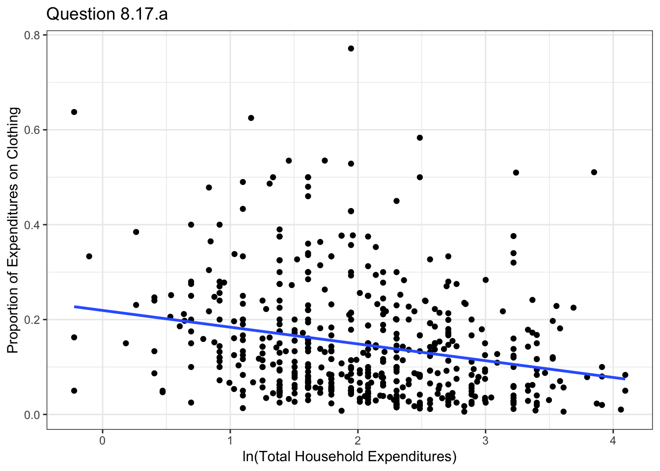

PCLOTHES versus ln(TOTEXP) with OLS fitted line

model17a <- lm(data=malawi, pclothes~lntotexp)

# write a function to obtain elasticity and confidence interval
elasticityCI <- function(x, y, value) {

  model_e <-lm(y~x)

  # Use mean value of totexp and estimates to calculate elasticity
  coef1 =  summary(model_e)$coefficients[1]
  coef2 =  summary(model_e)$coefficients[2]

  # compute elasticity
  e = (coef1 + coef2*(value+1))/(coef1 + coef2*(value))

  # Use delta method to obtain a confidence interval around this elasticity
  # first, obtain covariance matrix from regression output
  cov_mat = vcov(model_e)

  # get derivatives of elasticity with respect to each parameter in the model
  de_db1 = -coef2/(coef1 + coef2*value)^(2)
  de_db2 = coef1/(coef1 + coef2*value)^(2)

  # define matrix of derivatives
  D = matrix( nrow=1, ncol = 2)
  D[1, 1] = de_db1
  D[1, 2] = de_db2

  # get estimated variance matrix of the elasticity
  varmat = D%*% cov_mat %*%t(D)

  # obtain the standard error by taking the square room
  se = sqrt(varmat)

  # and finally, obtain the 95% confidence interval
  ub = e+1.96*se
  lb = e-1.96*se

  return(c(e, lb, ub))

}

# call function to obtain results
results17a = elasticityCI(malawi$lntotexp, malawi$pclothes, log(mean(malawi$totexp)))

The elasticity of clothing expenditures with respect to total expenditures at the mean is 0.741, with a confidence interval of [0.643, 0.84]. The elasticity is less than one, which makes sense since clothing is a necessary good.

b) Log-log model

Calculate \(CLOTHES = PCLOTHES \times TOTEXP\). Then plot ln(CLOTHES) versus ln(TOTEXP) and include the least squares fitted line. Calculate a 95% interval estimate of the elasticity of clothing expenditures with respect to total expenditures. Is the elasticity computed in part (a) within this interval?

# plot PCLOTHES versus TOTEXP and include the least squares fitted line.
malawi$clothes <- malawi$pclothes*malawi$totexp
malawi$lnclothes <- log(malawi$clothes)

# plot LNCLOTHES versus LNTOTEXP and include the least squares fitted line.
ggplot(data=malawi, aes(x=lntotexp , y=lnclothes))+geom_point() +
  geom_smooth(method = "lm", se = FALSE ,formula= y~x)+xlab("ln(Total Household Expenditures)")+
  ylab("ln(Total Expenditures on Clothing)")+theme_bw()+ggtitle("Question 8.17.b")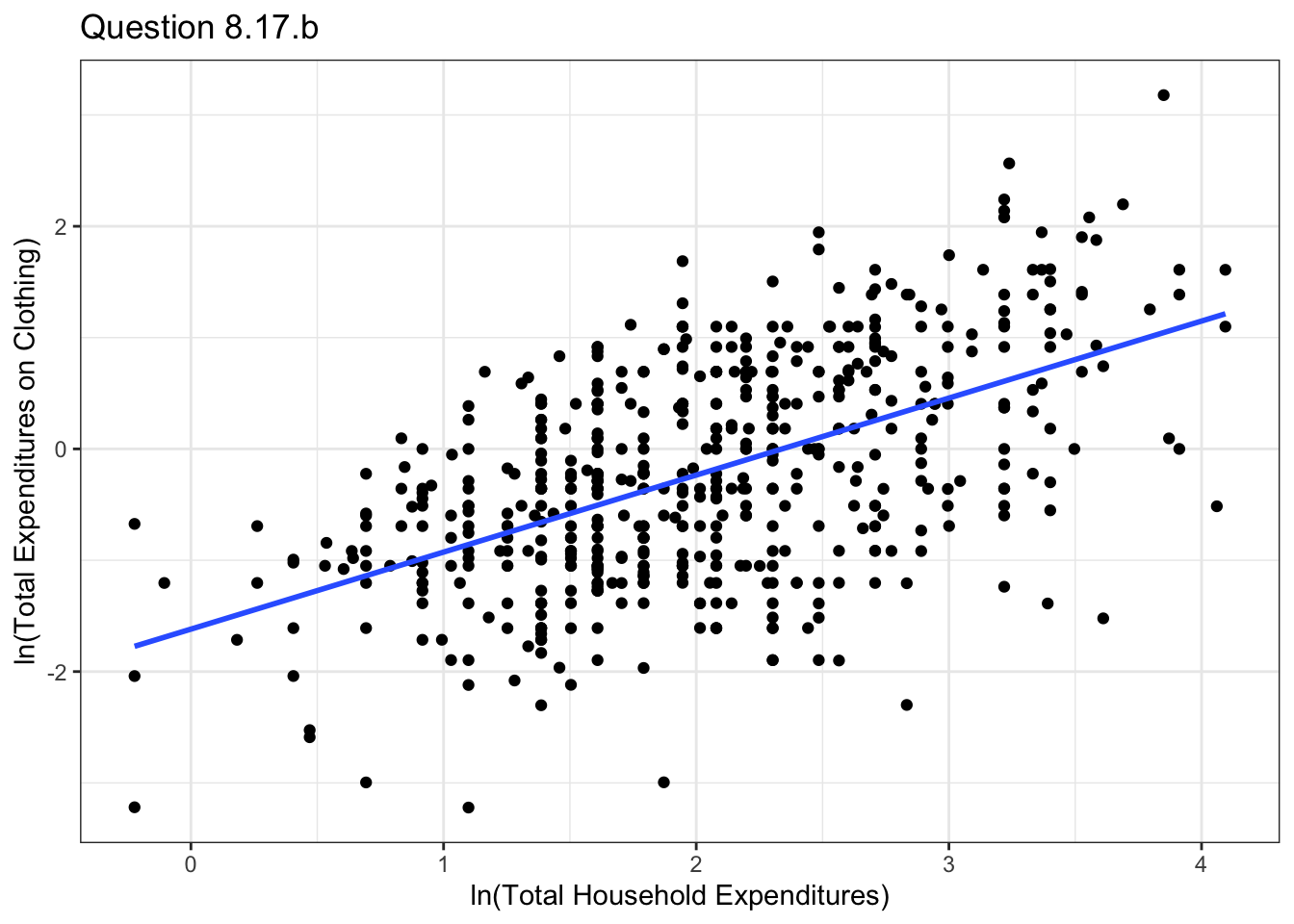

ln(CLOTHES) versus ln(TOTEXP) with OLS fitted line

# get the regression coefficient
model17b <- lm(data=malawi, lnclothes~lntotexp)
print(summary(model17b))

Call:
lm(formula = lnclothes ~ lntotexp, data = malawi)

Residuals:
    Min      1Q  Median      3Q     Max 
-2.6710 -0.6144  0.0675  0.6005  2.1330 

Coefficients:
            Estimate Std. Error t value Pr(>|t|)    
(Intercept)  -1.6186     0.0975   -16.6   <2e-16 ***
lntotexp      0.6918     0.0448    15.4   <2e-16 ***
---
Signif. codes:  0 '***' 0.001 '**' 0.01 '*' 0.05 '.' 0.1 ' ' 1

Residual standard error: 0.833 on 554 degrees of freedom
Multiple R-squared:  0.301, Adjusted R-squared:  0.299 
F-statistic:  238 on 1 and 554 DF,  p-value: <2e-16

# get confidence interval
lb17b = summary(model17b)$coefficients[2] - 1.96*coef(summary(model17b))[, 2][2]
ub17b = summary(model17b)$coefficients[2] + 1.96*coef(summary(model17b))[, 2][2]

The elasticity in this case is 0.692, with a confidence interval of [0.604, 0.78]. The elasticity computed in part (a) is within the interval.

c) Linear model

Plot CLOTHES versus TOTEXP and include the least squares fitted line. Calculate a 95% interval estimate of the elasticity of clothing expenditures with respect to total expenditures at the means. Is the elasticity computed in part (a) within this interval?

In this case, note that the elasticity is: \[\epsilon = \frac{d CLOTHES}{d TOTEXP}\frac{TOTEXP}{CLOTHES} = \hat{\gamma}_1 \cdot \frac{\overline{TOTEXP}}{\hat{\gamma}_1 +\hat{\gamma}_2 \overline{TOTEXP}}\] where \(\overline{TOTEXP}\) is the average of total expenditures.

# plot PCLOTHES versus TOTEXP and include the least squares fitted line.
ggplot(data=malawi, aes(x=totexp , y=clothes))+geom_point() +
  geom_smooth(method = "lm", se = FALSE ,formula= y~x)+xlab("Total Household Expenditures")+
  ylab("Total Expenditures on Clothing")+theme_bw()+ggtitle("Question 8.17.c")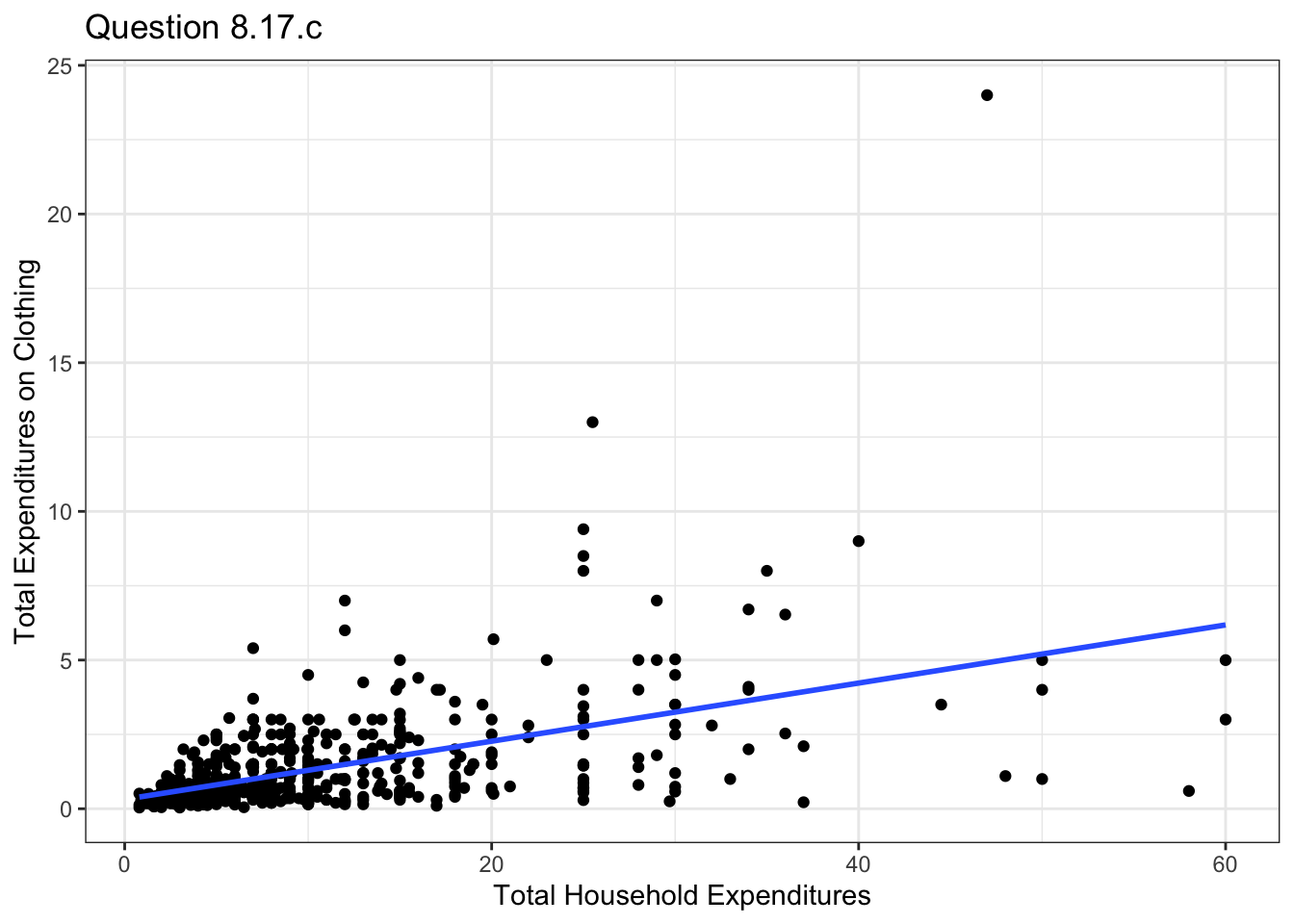

CLOTHES versus TOTEXP with OLS fitted line

# get the regression coefficient
model17c <- lm(data=malawi, clothes~totexp)

# get estimates
gamma1 = summary(model17c)$coefficients[1]
gamma2 = summary(model17c)$coefficients[2]
mean_totexp =  mean(malawi$totexp)

# get elasticity
e17c = gamma2*mean_totexp/(gamma1+gamma2*mean_totexp)

# Use delta method to obtain a confidence interval around this elasticity
# first, obtain covariance matrix from regression output
cov_mat = vcov(model17c)

# get derivatives of elasticity with respect to each parameter in the model
de_db117c = -gamma2*mean_totexp/(gamma1+gamma2*mean_totexp)^2
de_db217c = gamma1*mean_totexp/(gamma1+gamma2*mean_totexp)^2

# define matrix of derivatives
D17c = matrix( nrow=1, ncol = 2)
D17c[1, 1] = de_db117c
D17c[1, 2] = de_db217c

# get estimated variance matrix of the elasticity
varmat17c = D17c%*% cov_mat %*%t(D17c)

# obtain the standard error by taking the square room
se17c = sqrt(varmat17c)

# and finally, obtain the 95% confidence interval
ub17c = e17c+1.96*se17c[1]
lb17c = e17c-1.96*se17c[1]

The elasticity in this case is 0.763, with a confidence interval of [0.636, 0.889].

d) Breusch-Pagan tests for heteroskedasticity

Test for the presence of heteroskedasticity in each model in parts (a)–(c). Use the 1% level of significance. What are your conclusions? For which specification does heteroskedasticity seem less of an issue?

We compute the LM test for each model.

# for model (a)
bptest(model17a)

    studentized Breusch-Pagan test

data:  model17a
BP = 3.2, df = 1, p-value = 0.07

# for model (b)
bptest(model17b)

    studentized Breusch-Pagan test

data:  model17b
BP = 13, df = 1, p-value = 0.0003

# for model (c)
bptest(model17c)

    studentized Breusch-Pagan test

data:  model17c
BP = 45, df = 1, p-value = 2e-11

We find that heteroskedasticity appears to be an issue in models in parts (b) and (c), since in these cases we reject homoskedasticity at the 5% level.

e) Robust standard errors

For the models in which heteroskedasticity was significant at the 1% level, use OLS with robust standard errors. Calculate a 95% interval estimate for the elasticity of clothing expenditures with respect to total expenditures at the means. How do the intervals compare to the ones based on conventional standard errors?

Now we re-compute the confidence intervals using robust standard errors for models (b) and (c).

# get robust standard errors and confidence interval for model (b)
cov17b <- hccm(model17b, type="hc1")
robust_se17b <- coeftest(model17b, vcov.=cov17b)
robust_lb17b = summary(model17b)$coefficients[2] - 1.96*robust_se17b[2, 2]
robust_ub17b = summary(model17b)$coefficients[2] + 1.96*robust_se17b[2, 2]

# get robust standard errors and confidence interval for model (c)
cov17c <- hccm(model17c, type="hc1")
robust_varmat17c = D17c%*% cov17c  %*%t(D17c)

# obtain the standard error by taking the square room
robust_se17c = sqrt(robust_varmat17c)

# and finally, obtain the 95% confidence interval
robust_ub17c = e17c+1.96*robust_se17c[1]
robust_lb17c = e17c-1.96*robust_se17c[1]

For the log-log model in part (b) the elasticity interval estimate using the default robust standard error is [0.601, 0.783]. For the linear model in part (c) the elasticity interval becomes [0.533, 0.993]. For the log-log model the interval estimate is only slightly wider than using conventional OLS standard errors. For the linear model the interval estimate is much wider, which is to be expected given the strong heteroskedasticity in that model.

---

Question 8.21

In Example 8.9 we estimated the linear probability model: \[ COKE = \beta_1 + \beta_2 PRATIO + \beta_3 DISP\_COKE + \beta_4 DISP\_PEPSI + e\] where COKE = 1 if a shopper purchased Coke and COKE = 0 if a shopper purchased Pepsi. The variable PRATIO was the relative price ratio of Coke to Pepsi and DISP_COKE and DISP_PEPSI were indicator variables equal to one if the relevant display was present. Suppose now that we have 1140 observations on randomly selected shoppers from 50 different grocery stores. Each grocery store has its own settings for PRATIO, DISP_COKE and DISP_PEPSI. Let an \((i, j)\) subscript denote the jth shopper at the ith store, so that we can write the model as: \[ COKE_{ij} = \beta_1 + \beta_2 PRATIO_i + \beta_3 DISP\_COKE_i + \beta_4 DISP\_PEPSI_i + e_{ij}\] Average this equation over all shoppers in the ith store so that we have \[ \overline{COKE}_{i} = \beta_1 + \beta_2 PRATIO_i + \beta_3 DISP\_COKE_i + \beta_4 DISP\_PEPSI_i + \bar{e}_{i}\] where \(\bar{e}_{i} = \frac{1}{N_i}\sum_j e_{ij}\), \(\bar{COKE}_{i} = \frac{1}{N_i}\sum_j COKE_{ij}\), and \(N_i\) is the number of sampled shoppers in the \(i\)-th store.

a) Interpretation of \(\overline{COKE}_i\)

What is the interpretation of \(\overline{COKE}_i\) for the ith store?

\(\overline{COKE}_i\) is the share of shoppers in the \(i\)th store that purchased coke.

b) Conditional mean and variance

Assume that \(E\left(COKE_{ij} \vert x_{ij} \right) = P_i\) and \(\text{var}\left(COKE_{ij} \vert x_{ij} \right) = P_i(1-P_i)\), show \(E\left(\overline{COKE}_{i} \vert X \right) = P_i\) and \(\text{var}\left(\overline{COKE}_{i} \vert X \right) = P_i(1-P_i)/N_i\)

\[E\left(\overline{COKE}_{i} \vert X \right) = \frac{1}{N_i} E\left(\sum_j COKE_{ij} \vert X \right) =\frac{1}{N_i} N_i P_i = P_i \]

\[\text{var}\left(\overline{COKE}_{i} \vert X \right) = \frac{1}{N_i^2} \sum_j \text{var}\left(COKE_{ij} \vert X \right) + \text{zero covariance terms} =\frac{1}{N_i^2} N_i P_i(1-P_i)=\frac{ P_i(1-P_i)}{N_i} \]

c) Interpret \(P_i\)

Interpret \(P_i\) and express it in terms of \(PRATIO_i\), \(DISP\_COKE_i\), and \(DISP\_PEPSI_i\).

\(P_i\) is the population proportion of customers in store \(i\) who purchase Coke, or the probability that a customer in store \(i\) will purchase Coke. Given the model we have and our result from part (b) we can say that: \[ P_i = \beta_1 + \beta_2 PRATIO_i + \beta_3 DISP\_COKE_i + \beta_4 DISP\_PEPSI_i\]

d) Summary statistics and coefficients of variation

Observations on the variables \(\overline{COKE}_i, PRATIO_i, DISP\_COKE_i, DISP\_PEPSI_i\) and \(N_i\) appear in the data file coke_grouped. Obtain summary statistics for the data. Calculate the sample coefficient of variation for \(\bar{COKE}_{i}\) and \(PRATIO_{i}\). How much variation is there in these variables relative to their mean? Would we prefer larger or smaller coefficients of variation in these variables? Why? Construct histograms for these two variables. What do you observe?

# load in the dataset
coke_grouped <- read.csv("data/coke_grouped.csv")

# compute coefficient of variation
coke_CV = 100*sd(coke_grouped$coke_bar)/mean(coke_grouped$coke_bar)
pratio_CV = 100*sd(coke_grouped$pratio)/mean(coke_grouped$pratio)

The coefficient of variation for \(\overline{COKE}_i\) is 24.1875262653212% and for the price ratio is 4.92449354657242%. Based on these values as well as the histograms below, we can see that there is more variation in the share of consumers buying coke than in the price ratio. In most stores, the price of Coke is higher than the price of Pepsi.

stargazer(coke_grouped, type = "text")

=========================================
Statistic  N   Mean  St. Dev.  Min   Max 
-----------------------------------------
coke_bar   50 0.449   0.108   0.211 0.733
pratio     50 1.027   0.051   0.901 1.112
disp_coke  50 0.140   0.351     0     1  
disp_pepsi 50 0.140   0.351     0     1  
n          50 22.800  4.454    14    34  
-----------------------------------------

ggplot(coke_grouped, aes(x=coke_bar)) +
 geom_histogram(aes(y=after_stat(density)), colour="black", fill="white", bins=6)+
 geom_density(alpha=.2, fill="#FF6666") +xlab("Share of Shoppers Buying Coke") + theme_bw()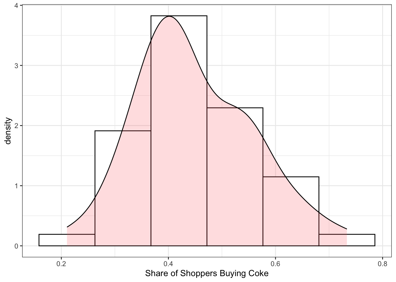

Distribution of share of shoppers buying Coke

ggplot(coke_grouped, aes(x=pratio)) +
 geom_histogram(aes(y=after_stat(density)), colour="black", fill="white", bins=6)+
 geom_density(alpha=.2, fill="#FF6666") +xlab("Price Ratio") + theme_bw()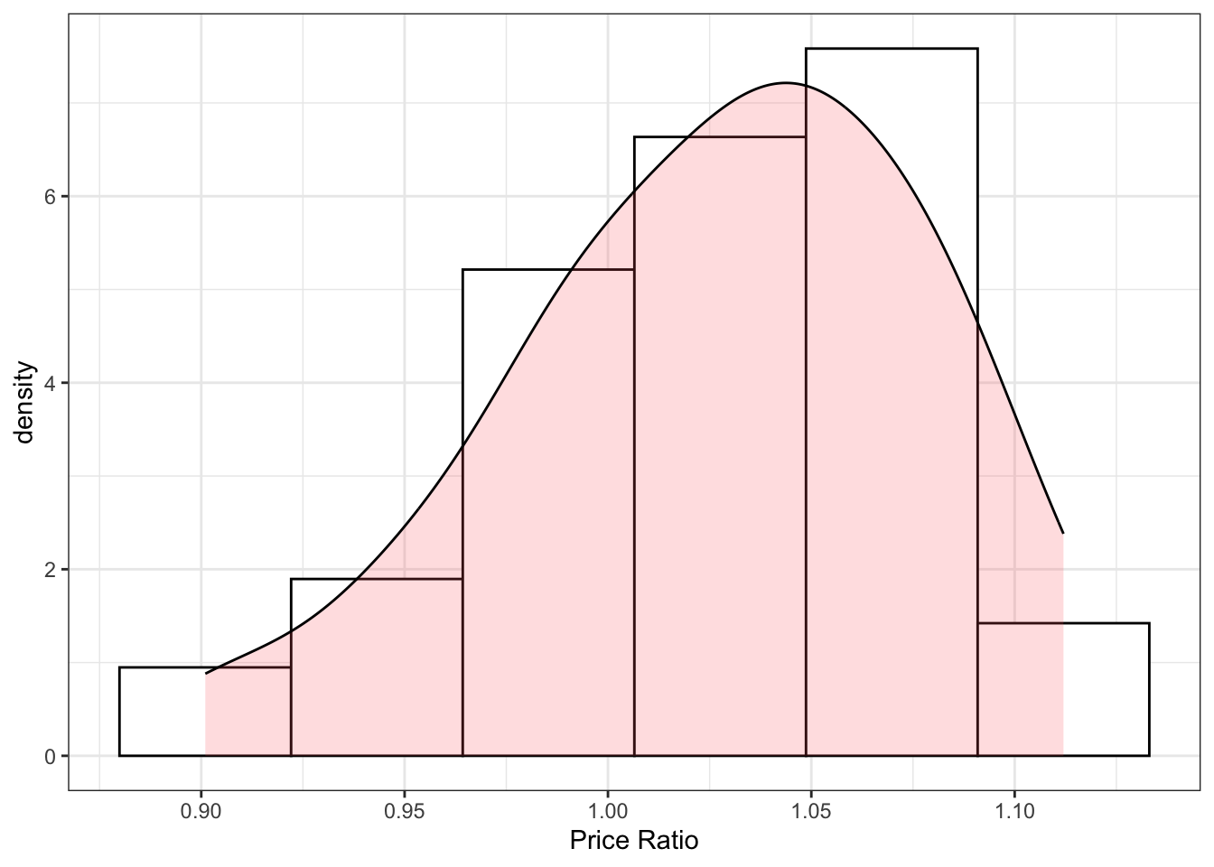

Distribution of price ratio

e) OLS with robust standard errors and hypothesis test

Find least squares estimates of equation above and use robust standard errors. Summarize the results. Test the null hypothesis \(\beta_3 = -\beta_4\). Choose an appropriate alternative hypothesis and use the 5% level of significance. If the null hypothesis is true, what does it imply about the effect of store displays for COKE and PEPSI?

# estimate regression model
model21e <- lm(data=coke_grouped, coke_bar ~ pratio + disp_coke + disp_pepsi)

# get robust standard errors
cov1 <- hccm(model21e, type="hc1")
robust_model21e = coeftest(model21e, vcov.=cov1)

# test statistic
t = (robust_model21e[3, 1] + robust_model21e[4, 1] ) /
     ( cov1[3, 3] + cov1[4, 4] + 2*cov1[4, 3] )^(1/2)

The alternative hypothesis is a two-sided test since it is that \(\beta_3 \neq -\beta_4\). The test statistic is -0.6, which is far below the 5% critical value level of 2.013.

f) White test and \(NR^2\) test

Create the variable \(DISP = DISP\_COKE - DISP\_PEPSI\). Estimate the model: \[\overline{COKE}_i =\beta_1 + \beta_2 PRATIO_i + \beta_3 DISP_i + e_i \] by OLS. Test for heteroskedasticity by applying the White test. Also carry out the \(NR^2\) test for heteroskedasticity using the candidate variable \(N_i\). What are your conclusions, at the 5% level?

# create new variable
coke_grouped$disp = coke_grouped$disp_coke - coke_grouped$disp_pepsi

# estimate regression model
model21f <- lm(data=coke_grouped, coke_bar ~ disp + pratio)
resid = residuals(model21f)^2

# white test
coke_grouped$pratiosq <- coke_grouped$pratio^2
coke_grouped$dispsq <- coke_grouped$disp^2
coke_grouped$interact <- coke_grouped$disp*coke_grouped$pratio

# estimate the regression of residuals on covariates
resid_model21f_1 = lm(resid~ coke_grouped$interact+coke_grouped$pratiosq+coke_grouped$pratio+
                        coke_grouped$dispsq+coke_grouped$disp)

# extract r2 and compute test stat
white_statistic = summary(resid_model21f_1)$r.squared*nrow(coke_grouped)

# get the critical value
# 6 parameters, null hypothesis sets 5 of them equal to 0
# so we have df = 5
white_cv = qchisq(0.95, df=5)

# NR2
# compute residuals
resid_model21f_2 = lm(resid~coke_grouped$n)
NR_statistic = summary(resid_model21f_2)$r.squared*nrow(coke_grouped)

# get the critical value
# 2 parameters, null hypothesis sets 1 of them equal to 0
# so we have df = 1
NR_cv = qchisq(0.95, df=1)

The White test statistic is 6.718. There are 6 parameters and the null hypothesis is that five them are equal to 0, so the critical value is 11.07. In this case, since the test statistic falls below the critical value, we fail to reject homoskedasticity. The NR test statistic is 4.666. There are 2 parameters and the null hypothesis is that one of them is equal to 0, so the critical value is 3.841. In this case thus we conclude that heteroskedasticity is present.

g) Fitted values and estimated variance

Obtain the fitted values from (e), \(p_i\), and estimate \(\text{var}(\overline{COKE}_i)\) for each of the stores. Report the mean, standard deviation, maximum and minimum values of the \(p_i\).

# estimate regression model
p <- model21e$coefficients[1] + model21e$coefficients[2]*coke_grouped$pratio +
  model21e$coefficients[3]*coke_grouped$disp_coke +model21e$coefficients[4]*coke_grouped$disp_pepsi

varcoke = p*(1-p)/coke_grouped$n

stargazer(data.frame(p), type = "text")

=======================================
Statistic N  Mean  St. Dev.  Min   Max 
---------------------------------------
p         50 0.449  0.041   0.339 0.546
---------------------------------------

---

Question 8.27

There were 64 countries who competed in the 1992 Olympics and won at least one medal. For each of these countries, let MEDALTOT be the total number of medals won, POP be population in millions, and GDP be GDP in billions of 1995 dollars.

a) OLS estimation

Use the data file olympics5, excluding the United Kingdom, and use the N = 63 remaining observations. Estimate the model: \(MEDALTOT = \beta_1 + \beta_2 \ln(POP) + \beta_3 \ln(GDP) + e\) by OLS.

olympics <- read.csv("data/olympics.csv")

# restrict the dataset to 1992 and include only countries who won at least one metal
olympics <- olympics[olympics$year==92,]
olympics <- olympics[olympics$medaltot>0 & !is.na(olympics$medaltot),]

# remove the UK (i.e. Great Britain)
olympics <- olympics[olympics$co_code!="GBR",]
olympics$gdp <- olympics$gdp/(10^9)
olympics$pop <- olympics$pop/(10^6)

# estimate the model
model27a <- lm(data=olympics, medaltot ~ log(pop) + log(gdp) )
print(summary(model27a))

Call:
lm(formula = medaltot ~ log(pop) + log(gdp), data = olympics)

Residuals:
   Min     1Q Median     3Q    Max 
-25.13 -12.79  -4.66   6.38  85.19 

Coefficients:
            Estimate Std. Error t value Pr(>|t|)    
(Intercept)   113.54      21.39    5.31  1.7e-06 ***
log(pop)        2.76       2.07    1.34    0.187    
log(gdp)        4.27       1.72    2.49    0.016 *  
---
Signif. codes:  0 '***' 0.001 '**' 0.01 '*' 0.05 '.' 0.1 ' ' 1

Residual standard error: 19.6 on 60 degrees of freedom
Multiple R-squared:  0.275, Adjusted R-squared:  0.251 
F-statistic: 11.4 on 2 and 60 DF,  p-value: 0.0000636

b) F-test and LM test for heteroskedasticity

Calculate the squared least squares residuals \(\hat{e}_i^2\) from the regression in (a). Regress \(\hat{e}_i^2\) on ln(POP) and ln(GDP). Use the F-test from this regression to test for heteroskedasticity at the 5% level of significance. Use the \(R^2\) from this regression to test for heteroskedasticity. What are the p-values of the two tests?

olympics$resid = residuals(model27a)^2
model27b <- summary(lm(data=olympics, resid~log(pop) + log(gdp)))

# get F-statistic
fstat_pval = pf(model27b$fstatistic[1],model27b$fstatistic[2],
                model27b$fstatistic[3],lower.tail=FALSE)

# get LM test statistic
NR_statistic = model27b$r.squared*nrow(olympics)
NR_pval = pchisq(NR_statistic, df=2, lower.tail=FALSE)

The F-statistic is 4.565 and the p-value is 0.014. Using this test we reject the null hypothesis of homoskedasticity at the 5% level. The value of the LM statistic is 8.321 and the p-value is 0.016. Using this test we reject the null hypothesis of homoskedasticity at the 5% level.

c) Robust standard errors and GDP hypothesis test

Reestimate the model in (a) but using heteroskedasticity robust standard errors. Using a 10% significance level, test the hypothesis that there is no relationship between the number of medals won and GDP against the alternative that there is a positive relationship. What happens if you change the significance level to 5%?

# estimate the model again
cov27c <- hccm(model27a, type="hc1")
robust_se27c <- coeftest(model27a, vcov.=cov27c)
print(robust_se27c)

t test of coefficients:

            Estimate Std. Error t value Pr(>|t|)   
(Intercept)   113.54      33.84    3.35   0.0014 **
log(pop)        2.76       1.79    1.55   0.1276   
log(gdp)        4.27       1.78    2.40   0.0195 * 
---
Signif. codes:  0 '***' 0.001 '**' 0.01 '*' 0.05 '.' 0.1 ' ' 1

tstat = robust_se27c[3, 1]/robust_se27c[3, 2]

t_cv10 = qt(.90, 60, lower.tail=TRUE)
t_cv5 = qt(.95, 60, lower.tail=TRUE)

The t-statistic is 2.399, which is larger than both the 10% critical value of 1.296 and the 5% critical value of 1.671. Thus, we conclude that there is a positive relationship between GDP and the expected number of medals won at either the 5% or 10% level of significance.

d) Population hypothesis test

Using a 10% significance level, test the hypothesis that there is no relationship between the number of medals won and population against the alternative that there is a positive relationship. What happens if you change the significance level to 5%?

# estimate the model again
tstat_pop = robust_se27c[2, 1]/robust_se27c[2, 2]

Using the regression results and critical values in part (c), we see that the test statistic is 2, which lies between the 5% and 10% critical values. Thus, we conclude that there is a positive relationship between the population size and the expected number of medals won at the 10% level of significance, but not at the 5% level.

e) Prediction for the United Kingdom

Use the model in (c) to find point and 95% interval estimates for the expected number of medals won by the United Kingdom whose population and GDP in 1992 were 58 million and $1010 billion, respectively.

expected_medals = summary(model27a)$coefficients[1, 1] + summary(model27a)$coefficients[2, 1]*
                  log(58)  +  summary(model27a)$coefficients[3, 1]*log(1010)

# get derivatives of elasticity with respect to each parameter in the model
de_db1 = 1
de_db2 = log(58)
de_db3 = log(1010)

# define matrix of derivatives
D = matrix( nrow=1, ncol = 3)
D[1, 1] = de_db1
D[1, 2] = de_db2
D[1, 3] = de_db3

# get estimated variance matrix of the elasticity
varmat = D%*% cov27c %*%t(D)

# obtain the standard error by taking the square room
se = sqrt(varmat)

# get confidence interval
ub27e = expected_medals + qt(.975, 60, lower.tail=TRUE)*se
lb27e = expected_medals - qt(.975, 60, lower.tail=TRUE)*se

The estimated expected number of medals won is 154.301. Using the delta method we find that the standard error is 46.836. The confidence interval is [60.615, 247.987].

f) Hypothesis test for UK prediction

The United Kingdom won 20 medals in 1992. Was the model successful in predicting the mean number of medals for the United Kingdom? Using the estimation in (c), with robust standard errors, what is the \(p\)-value for a test of \(H_0\): \(\beta_1 + \ln(58)\times \beta_2 + \ln(1010)\times \beta_3 = 20\) versus \(\beta_1 + \ln(58)\times \beta_2 + \ln(1010)\times \beta_3 \neq 20\).

Because 20 is inside the interval estimate from part (d), we will not reject the null hypothesis using a two-tail test at the 5% level.

---

Discussion Slides

Download Ch. 8 discussion slides (PDF)

Acknowledgements

Thank you to Coleman Cornell for generously sharing his materials with me.

---

1. The elasticity of expenditure on food with respect to total expenditure is \(\epsilon = \frac{\beta_1 + \beta_2 \left(\ln(TOTEXP)+1\right)}{\beta_1 + \beta_2 \ln(TOTEXP)}\)