Show code
newbroiler = read.csv("data/newbroiler.csv")Simultaneous Equations
These problems accompany Simultaneous Equations. Read that chapter first for the theory behind these exercises.
Suppose you want to estimate a wage equation for married women of the form
\[ \log(WAGE) = \beta_{1} + \beta_{2}HOURS + \beta_{3}EDUC + \beta_{4}EXPER + \beta_{5}EXPER^{2} + e_{1} \]
where \(WAGE\) is the hourly wage, \(HOURS\) is number of hours worked per week, \(EDUC\) is years of education, and \(EXPER\) is years of experience. Your classmate observes that higher wages can bring forth increased work effort, and that married women with small children may reduce their hours of work to take care of them. It may also be true that a husband’s wage rate has an effect on a wife’s hours of work supplied, so that there may be an auxiliary relationship such as
\[ HOURS = \alpha_{1} + \alpha_{2}\log(WAGE) + \alpha_{3}KIDS + \alpha_{4}\log(HWAGE) + e_{2} \]
where \(KIDS\) is the number of children under the age of six in the woman’s household and \(HWAGE\) is her husband’s wage rate.
Can the wage equation be estimated satisfactorily using the OLS estimator? If not, why not?
The wage equation cannot be satisfactorily estimated with the OLS estimator as there will be endogeneity bias on the estimate of \(\beta_{2}\) if the proposed auxiliary relationship is true.
Is the wage equation “identified”? What does the term identification mean in this context?
The wage equation is identified. In order to be identified, there needs to be at least one instrument that allows us to shift hours worked without directly impacting wages. In this example, we have the additional instruments of \(KIDS\) and \(HWAGE\), which should satisfy this requirement.
If you seek an alternative to least squares estimation for the wage equation, suggest an estimation procedure and how (step by step, and NOT a computer command) it is carried out.
The alternative is the Two Stage Least Squares
Estimate the reduced form equation for \(HOURS\): \[ HOURS = \theta_{1} + \theta_{2}EDUC + \theta_{3}EXPER + \theta_{4}EXPER^{2} + \theta_{5}KIDS + \theta_{6}\log(HWAGE) + u_{2} \]
Obtain fitted values \(\hat{HOURS}\) from this reduced form equation
Estimate the wage equation replacing \(HOURS\) with the fitted values from the reduced form equation.
Other than the identification condition in part (b), are there any other conditions that must be met so that we can confidently use the estimation procedure in part (c)? What are those conditions?
The other condition is that \(\theta_{5}\) and \(\theta_{6}\) are jointly significant must produce an \(F\)-stat large enough for the two instruments to be strong. If they are not strong, then the IVs are not able to shift the desired hours of work enough to estimate the true relationship between hours and wages.
This exercise examines a supply and demand model for edible chicken, which the U.S. Department of Agriculture calls “broilers.” The data for this exercise are in the file
newbroiler, which is adapted from the data provided by Epple and McCallum (2006). We consider the demand equation in this exercise and the supply equation in Exercise 11.21.
newbroiler = read.csv("data/newbroiler.csv")Consider the demand equation:
\[ \log(Q_{t}) = \alpha_{1} + \alpha_{2}\log(P_{t}) + \alpha_{3}\log(Y_{t}) + \alpha_{4}\log(PB_{t}) + \alpha_{5}POPGRO_{t} + e_{t}^{d} \]
where \(Q\) is the per capita consumption of chicken, in pounds; \(Y\) is real per capita income; \(P\) is the real price of chicken; \(PB\) is the real price of beef; and \(POPGRO\) is the rate of population growth. What are the endogenous variables? What are the exogenous variables?
Price \(P\) and quantity \(Q\) are the two endogenous variables in this regression. Real per capita income \(Y\), real price of beef \(PB\), and population growth \(POPGRO\) are the exogenous variables.
Using data from 1960 to 1999, estimate the demand equation by OLS. Comment on the signs and significance of the estimates.
ols.reg = dynlm(formula = log(q) ~ log(p) + log(y) + log(pb) + popgro,
                data = newbroiler[11:50,])
summary(ols.reg)
Time series regression with "numeric" data:
Start = 1, End = 40

Call:
dynlm(formula = log(q) ~ log(p) + log(y) + log(pb) + popgro,
    data = newbroiler[11:50, ])

Residuals:
     Min       1Q   Median       3Q      Max
-0.08954 -0.02680 -0.00088  0.02688  0.07776

Coefficients:
            Estimate Std. Error t value Pr(>|t|)
(Intercept)  -6.2325     0.7005   -8.90  1.6e-10 ***
log(p)       -0.1548     0.0864   -1.79    0.082 .
log(y)        0.9902     0.0693   14.28  3.6e-16 ***
log(pb)      -0.1553     0.0927   -1.68    0.103
popgro        0.1704     0.0355    4.80  2.9e-05 ***
---
Signif. codes:  0 '***' 0.001 '**' 0.01 '*' 0.05 '.' 0.1 ' ' 1

Residual standard error: 0.0428 on 35 degrees of freedom
Multiple R-squared:  0.981, Adjusted R-squared:  0.979
F-statistic:  450 on 4 and 35 DF,  p-value: <2e-16
The coefficient on log price is negative, but not significant. The coefficient on log income is positive and significant. The coefficient on the price of beef is negative, but not significant. The coefficient on population growth is positive and significant.
Test the OLS residuals from part (b) for serial correlation by constructing a correlogram and carrying out the \(T \times R^{2}\) test. What do you conclude about the presence of serial correlation?
resid.ts = ts(residuals(ols.reg))
acf(resid.ts, main = "Residual ACF")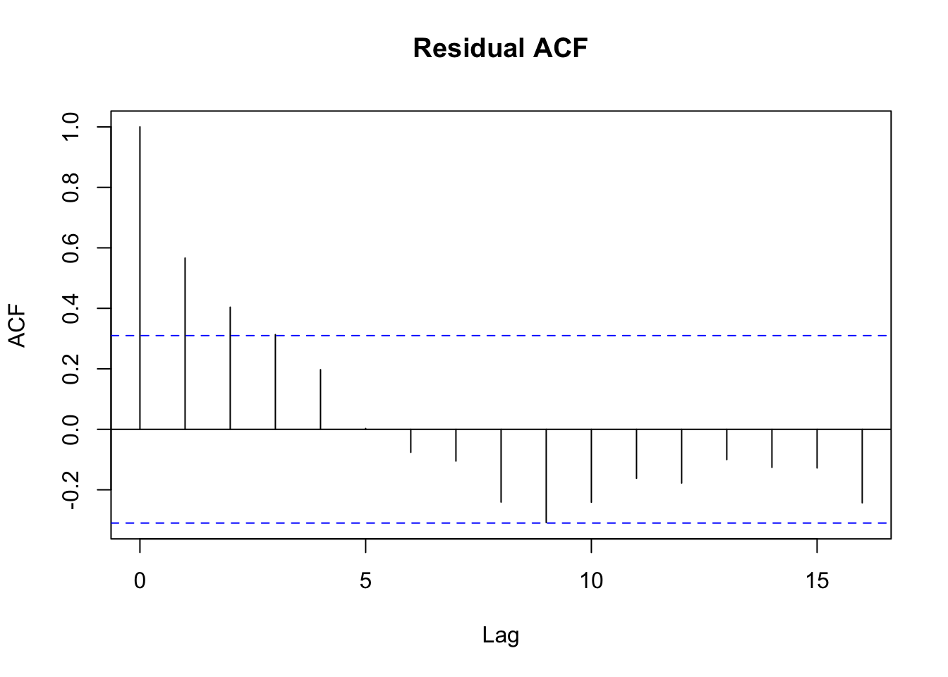
The correlogram indicates that there may be autocorrelation at the first and second lag.
lm.test = dynlm(resid.ts ~ L(resid.ts,1:2))
summary(lm.test)
Time series regression with "ts" data:
Start = 3, End = 40

Call:
dynlm(formula = resid.ts ~ L(resid.ts, 1:2))

Residuals:
     Min       1Q   Median       3Q      Max
-0.05495 -0.02097 -0.00164  0.02125  0.05957

Coefficients:
                  Estimate Std. Error t value Pr(>|t|)
(Intercept)        0.00142    0.00484    0.29  0.77160
L(resid.ts, 1:2)1  0.65196    0.16451    3.96  0.00035 ***
L(resid.ts, 1:2)2  0.03350    0.15358    0.22  0.82858
---
Signif. codes:  0 '***' 0.001 '**' 0.01 '*' 0.05 '.' 0.1 ' ' 1

Residual standard error: 0.0298 on 35 degrees of freedom
Multiple R-squared:  0.443, Adjusted R-squared:  0.412
F-statistic: 13.9 on 2 and 35 DF,  p-value: 0.0000353
From the BG test of 2 lags, we have an \(N \times R^{2}\) test statistic of 17.732842. This is much greater than the critical value of 5.991465. Thus, we reject the null hypothesis of no serial correlation.
Estimate the demand equation by 2SLS using as instruments \(\log(PF_{t})\), \(TIME_{T} = YEAR_{t} - 1949\), \(\log(QPROD_{t - 1})\), and \(\log(EXPTS_{t - 1})\). Compare and contrast these estimates to the OLS estimates in part (a).
newbroiler[,"time"] = newbroiler[,"year"] - 1949
newbroiler[-1,"l.qprod"] = newbroiler[-52,"qprod"]
newbroiler[-1,"l.lexpts"] = newbroiler[-52,"lexpts"]

reg.2sls = ivreg(formula = log(q) ~ log(p) + log(y) + log(pb) + popgro | log(pf) + time
+ log(l.qprod) + l.lexpts + log(y) + log(pb) + popgro, data = newbroiler[11:50,])
summary(reg.2sls)
Call:
ivreg(formula = log(q) ~ log(p) + log(y) + log(pb) + popgro |
    log(pf) + time + log(l.qprod) + l.lexpts + log(y) + log(pb) +
        popgro, data = newbroiler[11:50, ])

Residuals:
      Min        1Q    Median        3Q       Max
-0.082779 -0.034047 -0.000115  0.035174  0.085203

Coefficients:
            Estimate Std. Error t value Pr(>|t|)
(Intercept)  -5.3594     1.0481   -5.11  1.1e-05 ***
log(p)       -0.2960     0.1514   -1.95    0.059 .
log(y)        0.9028     0.1043    8.65  3.2e-10 ***
log(pb)      -0.0998     0.1075   -0.93    0.359
popgro        0.1660     0.0370    4.48  7.5e-05 ***

Diagnostic tests:
                 df1 df2 statistic  p-value
Weak instruments   4  32      4.31   0.0067 **
Wu-Hausman         1  34      1.46   0.2356
Sargan             3  NA     24.27 0.000022 ***
---
Signif. codes:  0 '***' 0.001 '**' 0.01 '*' 0.05 '.' 0.1 ' ' 1

Residual standard error: 0.0444 on 35 degrees of freedom
Multiple R-Squared: 0.979,  Adjusted R-squared: 0.977
Wald test:  419 on 4 and 35 DF,  p-value: <2e-16
The new price elasticity (\(\alpha_{2}\)) is now estimated to be negative and is significant at the \(10\%\) level. This matches the expected relationship between price and quantities. The other variables have not been affected, which is expected.
Estimate the reduced-form, first-stage, equation and test the joint significance of \(\log(PF_{t})\), \(TIME_{t}\), \(\log(QPROD_{t - 1})\), and \(\log(EXPTS_{t - 1})\). Can we conclude that at least one instrument is strong?
stage1.reg = lm(log(p) ~ log(pf) + time + log(l.qprod) + l.lexpts + log(y) + log(pb) + popgro,
                data = newbroiler[11:50,])
stage1.reg.restricted = lm(log(p) ~ log(y) + log(pb) + popgro, data = newbroiler[11:50,])
summary(stage1.reg)
Call:
lm(formula = log(p) ~ log(pf) + time + log(l.qprod) + l.lexpts +
    log(y) + log(pb) + popgro, data = newbroiler[11:50, ])

Residuals:
     Min       1Q   Median       3Q      Max
-0.12927 -0.04200 -0.00833  0.04036  0.14963

Coefficients:
             Estimate Std. Error t value Pr(>|t|)
(Intercept)   -7.0670     6.2192   -1.14   0.2643
log(pf)        0.2002     0.1076    1.86   0.0720 .
time          -0.0519     0.0217   -2.39   0.0230 *
log(l.qprod)  -0.1365     0.3302   -0.41   0.6821
l.lexpts       2.1226     0.6975    3.04   0.0047 **
log(y)         1.0184     0.6226    1.64   0.1117
log(pb)        0.1478     0.2292    0.64   0.5236
popgro         0.0685     0.0941    0.73   0.4722
---
Signif. codes:  0 '***' 0.001 '**' 0.01 '*' 0.05 '.' 0.1 ' ' 1

Residual standard error: 0.0706 on 32 degrees of freedom
Multiple R-squared:  0.91,  Adjusted R-squared:  0.89
F-statistic: 46 on 7 and 32 DF, p-value: 6.34e-15SSE_U = sum(residuals(stage1.reg)^2)
SSE_R = sum(residuals(stage1.reg.restricted)^2)
Fstat = (SSE_R/SSE_U - 1)*((40 - 8)/4)
cF = qf(0.95,4,32)The \(F\) statistic for our test of joint significance is \(4.311655\), which is greater than the critical value of \(2.668437\). However, this is significantly smaller than the rule-of-thumb strength level of \(F > 10\). Thus, the set of instruments would not lead to confident results.
Test the reduced-form equation for serial correlation using the \(T \times R^{2}\) test.
stage1.resid.ts = ts(resid(stage1.reg))
lm.test = dynlm(stage1.resid.ts ~ L(stage1.resid.ts,1:2))
summary(lm.test)
Time series regression with "ts" data:
Start = 3, End = 40

Call:
dynlm(formula = stage1.resid.ts ~ L(stage1.resid.ts, 1:2))

Residuals:
    Min      1Q  Median      3Q     Max
-0.0869 -0.0419 -0.0144  0.0460  0.1709

Coefficients:
                          Estimate Std. Error t value Pr(>|t|)
(Intercept)               0.000406   0.009857    0.04    0.967
L(stage1.resid.ts, 1:2)1  0.435890   0.174111    2.50    0.017 *
L(stage1.resid.ts, 1:2)2 -0.011333   0.172030   -0.07    0.948
---
Signif. codes:  0 '***' 0.001 '**' 0.01 '*' 0.05 '.' 0.1 ' ' 1

Residual standard error: 0.0606 on 35 degrees of freedom
Multiple R-squared:  0.173, Adjusted R-squared:  0.126
F-statistic: 3.67 on 2 and 35 DF,  p-value: 0.0358
From the BG test of 2 lags, we have an \(N \times R^{2}\) test statistic of 6.931827. This is much greater than the critical value of 5.991465. Thus, we reject the null hypothesis of no serial correlation.
Estimate the reduced-form, first-stage, equation using HAC standard errors and test the joint significance of \(\log(PF_{t})\), \(TIME_{t}\), \(\log(QPROD_{t - 1})\), and \(\log(EXPTS_{t - 1})\).
stage1.HAC = coeftest(stage1.reg, vcov = NeweyWest)
stage1.HAC
t test of coefficients:

             Estimate Std. Error t value Pr(>|t|)
(Intercept)  -7.06703   45.72037  -0.155   0.8781
log(pf)       0.20025    0.75755   0.264   0.7932
time         -0.05190    0.15013  -0.346   0.7318
log(l.qprod) -0.13646    1.17118  -0.117   0.9080
l.lexpts      2.12255    0.94750   2.240   0.0322 *
log(y)        1.01837    4.10402   0.248   0.8056
log(pb)       0.14782    1.16615   0.127   0.8999
popgro        0.06846    0.42321   0.162   0.8725
---
Signif. codes:  0 '***' 0.001 '**' 0.01 '*' 0.05 '.' 0.1 ' ' 1
The estimated standard errors are much larger than with standard OLS standard errors. The coefficient on \(TIME\) is no longer significant, but the coefficient on lagged \(\log(EXPTS)\) is. The \(F\) test of joint significance is equivalent as part (e) as this test is based on coefficient estimates and not standard error estimates. Applying HAC standard errors only affects standard errors.
Obtain the 2SLS residuals from part (d). Construct a correlogram. Is there evidence of serial correlation? Obtain 2SLS estimates with HAC standard errors and compare the results to those in (d).
resid.2sls = ts(residuals(reg.2sls))
acf(resid.2sls)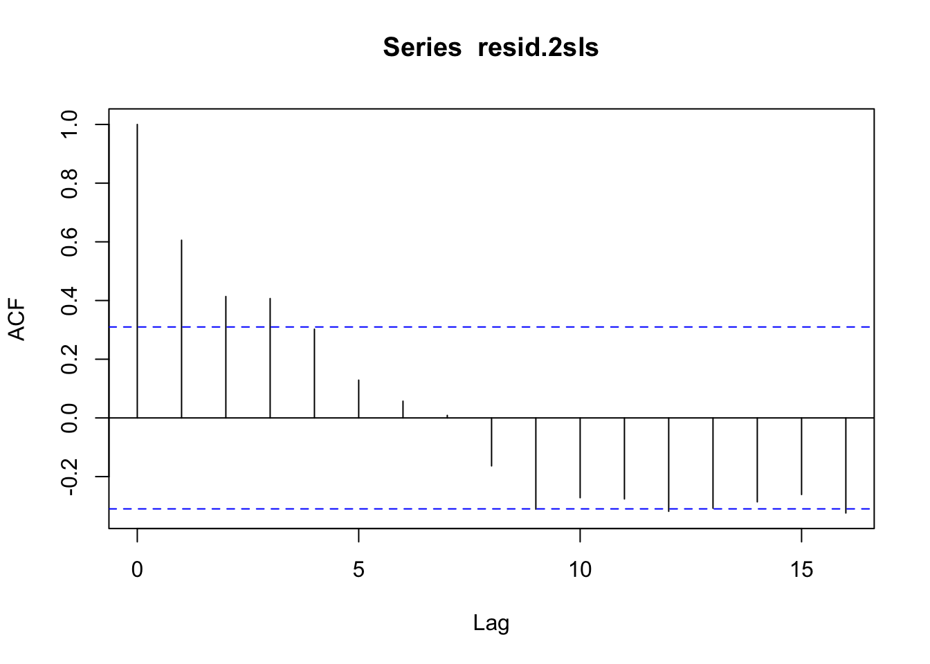
The correlogram indicates that there is significant autocorrelation at the first lag, while the second and third lags are potentially significant.
HAC.2sls = coeftest(reg.2sls, vcov = NeweyWest)
HAC.2sls
t test of coefficients:

            Estimate Std. Error t value Pr(>|t|)
(Intercept)  -5.3594     1.7535  -3.056  0.00427 **
log(p)       -0.2960     0.2364  -1.252  0.21898
log(y)        0.9028     0.1705   5.294 6.58e-06 ***
log(pb)      -0.0998     0.1354  -0.737  0.46591
popgro        0.1660     0.0747   2.223  0.03278 *
---
Signif. codes:  0 '***' 0.001 '**' 0.01 '*' 0.05 '.' 0.1 ' ' 1
The standard errors for all coefficients have increased, which is expected from a model that suffers from autocorrelation. The coefficient on the price of chickens is no longer significant at the \(10\%\) level, but the (lack of) significance for all other coefficients is unchanged.
Test the validity of the surplus instruments using the Sargan test, discussed in Section 10.4.3, and the 2SLS estimates in part (d).
The result of the Sargan test was shown earlier in the code output from part (d). The Sargan test statistic is 22.4073, with a \(p\)-value that is nearly zero. This means that one or more of the IVs are invalid, which potentially negates all the 2SLS results.
Supply and demand curves as traditionally drawn in economics principles classes have price (\(P\)) on the vertical axis and quantity (\(Q\)) on the horizontal axis.
Rewrite the truffle demand and supply equations in (11.11) and (11.12) with price \(P\) on the left-hand side. What are the anticipated signs of the parameters in this rewritten system of equations?
\[\begin{align} \text{Demand: } P_{i} &= \alpha_{1} + \alpha_{2}Q_{i} + \alpha_{3}PS_{i} + \alpha_{4}DI_{i} + e_{di}\\ \text{Supply: } P_{i} &= \beta_{1} + \beta_{2}Q_{i} + \beta_{3}PF_{i} + e_{si} \end{align}\]
where \(P\) is the market price of truffles, \(Q\) is the quantity of truffles traded in a particular French marketplace, \(PS\) is the market price of a substitute for real truffles (another fungus much less highly prized), and \(DI\) is per capita monthly disposable income of local residents, and \(PF\) is the hourly rental price of truffle-pigs used in the search process. Marketplaces are indexed by \(i\).
For the demand equation, we would anticipate that \(\alpha_{2}\) would be negative as the effect of scarcity on price would be reduced. We would anticipate \(\alpha_{3}\) to be positive as people would be willing to pay more for truffles if the substitute was more expensive as well. We would anticipate \(\alpha_{4}\) to be positive as individuals with higher disposable income might be willing to pay more for the same good.
For the supply equation, we would anticipate that \(\beta_{2}\) would be positive. We anticipate that \(\beta_{3}\) is positive as increasing the price of production would increase the price of the final good.
Using the data in the file
truffles, estimate the supply and demand equations that you have formulated in (a) using two-stage least squares. Are the signs correct? Are the estimated coefficients significantly different from zero?
truffles = read.csv("data/truffles.csv")
demand.2sls = ivreg(p ~ q + ps + di | pf + ps + di, data = truffles)
summary(demand.2sls)
Call:
ivreg(formula = p ~ q + ps + di | pf + ps + di, data = truffles)

Residuals:
   Min     1Q Median     3Q    Max
-39.66  -6.78   2.41   8.32  20.25

Coefficients:
            Estimate Std. Error t value Pr(>|t|)
(Intercept)   -11.43      13.59   -0.84   0.4081
q              -2.67       1.17   -2.27   0.0315 *
ps              3.46       1.12    3.10   0.0046 **
di             13.39       2.75    4.87 0.000047 ***

Diagnostic tests:
                 df1 df2 statistic p-value
Weak instruments   1  26      17.5 0.00029 ***
Wu-Hausman         1  25     120.0 4.9e-11 ***
Sargan             0  NA        NA      NA
---
Signif. codes:  0 '***' 0.001 '**' 0.01 '*' 0.05 '.' 0.1 ' ' 1

Residual standard error: 13.2 on 26 degrees of freedom
Multiple R-Squared: 0.557,  Adjusted R-squared: 0.506
Wald test: 17.4 on 3 and 26 DF,  p-value: 2.14e-06
The signs on all estimated slope coefficients in the demand equation are correct and significant.
supply.2sls = ivreg(p ~ q + pf | pf + ps + di, data = truffles)
summary(supply.2sls)
Call:
ivreg(formula = p ~ q + pf | pf + ps + di, data = truffles)

Residuals:
   Min     1Q Median     3Q    Max
-9.798 -2.344 -0.628  2.435 11.160

Coefficients:
            Estimate Std. Error t value Pr(>|t|)
(Intercept)  -58.798      5.859   -10.0  1.3e-10 ***
q              2.937      0.216    13.6  1.3e-13 ***
pf             2.958      0.156    19.0  < 2e-16 ***

Diagnostic tests:
                 df1 df2 statistic p-value
Weak instruments   2  26     28.93 2.4e-07 ***
Wu-Hausman         1  26      7.05   0.013 *
Sargan             1  NA      1.54   0.214
---
Signif. codes:  0 '***' 0.001 '**' 0.01 '*' 0.05 '.' 0.1 ' ' 1

Residual standard error: 4.4 on 27 degrees of freedom
Multiple R-Squared: 0.949,  Adjusted R-squared: 0.945
Wald test:  233 on 2 and 27 DF,  p-value: <2e-16
The signs on all estimated slope coefficients in the supply equation are correct and significant.
Estimate the price elasticity of demand “at the means” using the results from (b).
The price elasticity of demand “at the means” is equal to the following equation: \[ e_{p} = \frac{\Delta Q}{\Delta P}\frac{\bar{P}}{\bar{Q}} = \frac{1}{\alpha_{2}}\frac{\bar{P}}{\bar{Q}} \] The calculated value for this elasticity is -1.272464.
Accurately sketch the supply and demand equations, with \(P\) on the vertical axis and \(Q\) on the horizontal axis, using the estimates from part (b). For these sketches set the values of the exogenous variables \(DI\), \(PS\), and \(PF\) to be \(DI^{*} = 3.5\), \(PF^{*} = 23\), and \(PS^{*} = 22\).
price_seq = seq(5,30,1)
Demand = (demand.2sls$coefficients[[1]]
      + demand.2sls$coefficients[[2]] * price_seq
      + demand.2sls$coefficients[[3]] * 22
      + demand.2sls$coefficients[[4]] * 3.5)

Supply = (supply.2sls$coefficients[[1]]
      + supply.2sls$coefficients[[2]] * price_seq
      + supply.2sls$coefficients[[3]] * 23)

ggplot.df <- data.frame(price_seq,Demand,Supply)
ggplot.df <- melt(ggplot.df, id = "price_seq")

ggplot(data = ggplot.df, aes(x = price_seq,y = value, color = variable)) +
  xlim(5,30) + ylim(25,100) +
  ylab('Quantity') + xlab('Price') +
  geom_line()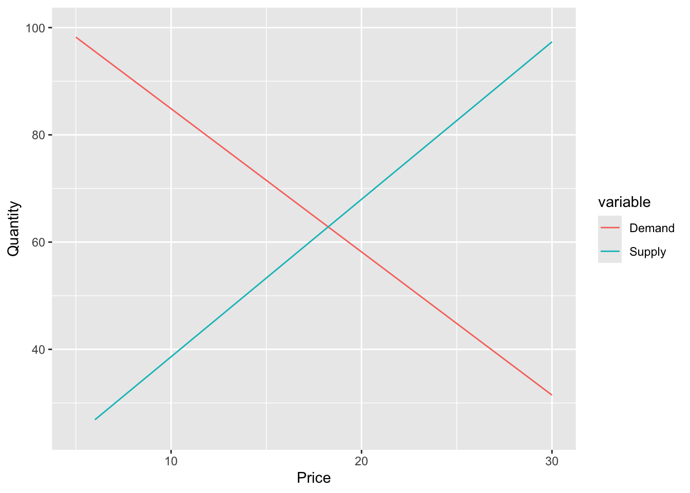
What are the equilibrium values of \(P\) and \(Q\) obtained in part (d)? Calculate the predicted equilibrium values of \(P\) and \(Q\) using the estimated reduced-form equations from Table 11.2, using the same values of the exogenous variables. How well do they agree?
The estimated equilibrium values from part (d) are computed by equating the supply and demand equations. After substituting in the given exogenous variables and estimated coefficients, we have the following equation to solve for the equilibrium: \[ 111.5801 - 2.6705Q_{EQM} = 9.2470 + 2.9367Q_{EQM} \] Solving for equilibrium quantity yields:
\[ Q_{EQM} = 18.2503 \]
To solve for equilibrium price, we then plug this in to either the supply or demand equations. Choosing the demand equation: \[ P_{EQM} = 111.5801 - 2.6705 \times 18.2503 = 62.8427 \]
Now, we compare to the reduced form predictions from Table 11.2:
\[\begin{align*} Q_{RF} &= 7.8951 * 0.6564 \times 22 + 2.1672 \times 3.5 - 0.5070 \times 23 = 18.2604\\ P_{RF} &= -32.5124 * 1.7081 \times 22 + 7.6025 \times 3.5 + 1.3539 \times 23 = 62.8154\\ \end{align*}\]
These results are almost identical to the calculated equilibrium results.
Estimate the supply and demand equations that you have formulated in (a) using OLS. Are the signs correct? Are the estimated coefficients significantly different from zero? Compare the results to those in part (b).
demand.ols = lm(p ~ q + ps + di, data = truffles)
summary(demand.ols)
Call:
lm(formula = p ~ q + ps + di, data = truffles)

Residuals:
   Min     1Q Median     3Q    Max
-25.07  -2.77  -0.41   4.71  17.50

Coefficients:
            Estimate Std. Error t value Pr(>|t|)
(Intercept)  -13.619      9.087   -1.50     0.15
q              0.151      0.499    0.30     0.76
ps             1.361      0.594    2.29     0.03 *
di            12.358      1.825    6.77  3.5e-07 ***
---
Signif. codes:  0 '***' 0.001 '**' 0.01 '*' 0.05 '.' 0.1 ' ' 1

Residual standard error: 8.81 on 26 degrees of freedom
Multiple R-squared:  0.801, Adjusted R-squared:  0.778
F-statistic:   35 on 3 and 26 DF,  p-value: 2.84e-09
The sign of the coefficient on \(Q\) has flipped from negative to positive, and is now incorrect. This suggests that individuals demand higher priced products more. In addition, the estimate is no longer significant. The magnitude of the coefficient on \(PS\) has also dropped.
supply.ols = lm(p ~ q + pf, data = truffles)
summary(supply.ols)
Call:
lm(formula = p ~ q + pf, data = truffles)

Residuals:
   Min     1Q Median     3Q    Max
-8.472 -3.329  0.186  2.078 10.751

Coefficients:
            Estimate Std. Error t value Pr(>|t|)
(Intercept)  -52.876      5.024   -10.5  4.7e-11 ***
q              2.661      0.171    15.5  5.4e-15 ***
pf             2.922      0.148    19.7  < 2e-16 ***
---
Signif. codes:  0 '***' 0.001 '**' 0.01 '*' 0.05 '.' 0.1 ' ' 1

Residual standard error: 4.2 on 27 degrees of freedom
Multiple R-squared:  0.953, Adjusted R-squared:  0.95
F-statistic:  274 on 2 and 27 DF,  p-value: <2e-16
The estimates in the supply equation are similar to before, and are all significantly different from zero.
Thank you to Coleman Cornell for generously sharing his materials with me.