19 The Tobit Model
Censored Regression for Data with a Pile-Up at Zero
Many economic outcomes bunch at zero: charitable donations, hours of overtime, spending on durable goods. The zeros are not missing data, they represent a corner solution. OLS on all observations pulls the slope toward zero; OLS on positives only ignores the participation decision. The Tobit model combines both through a latent variable framework and maximum likelihood estimation.
This page is part of the Qualitative and Limited Dependent Variable Models sequence. You should be comfortable with the latent variable framework and maximum likelihood estimation from Binary Choice Models before continuing.
19.1 A Spike at Zero
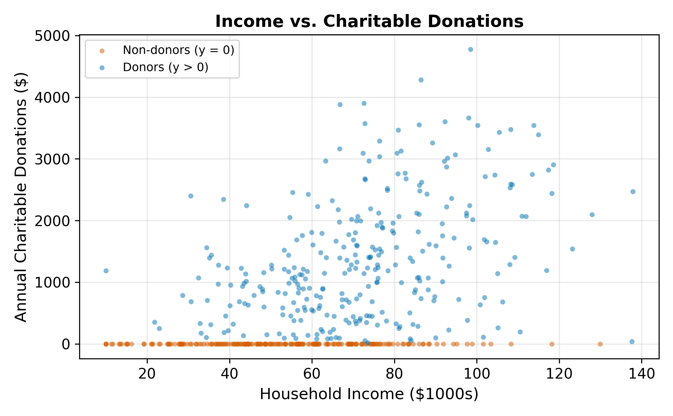
Consider modeling charitable donations. We observe a sample of households with data on annual donations (\(y_i\)), household income, years of education, and number of children. A histogram of donations reveals a striking pattern: a large fraction of households donate exactly zero, with the remaining observations spread across positive values.
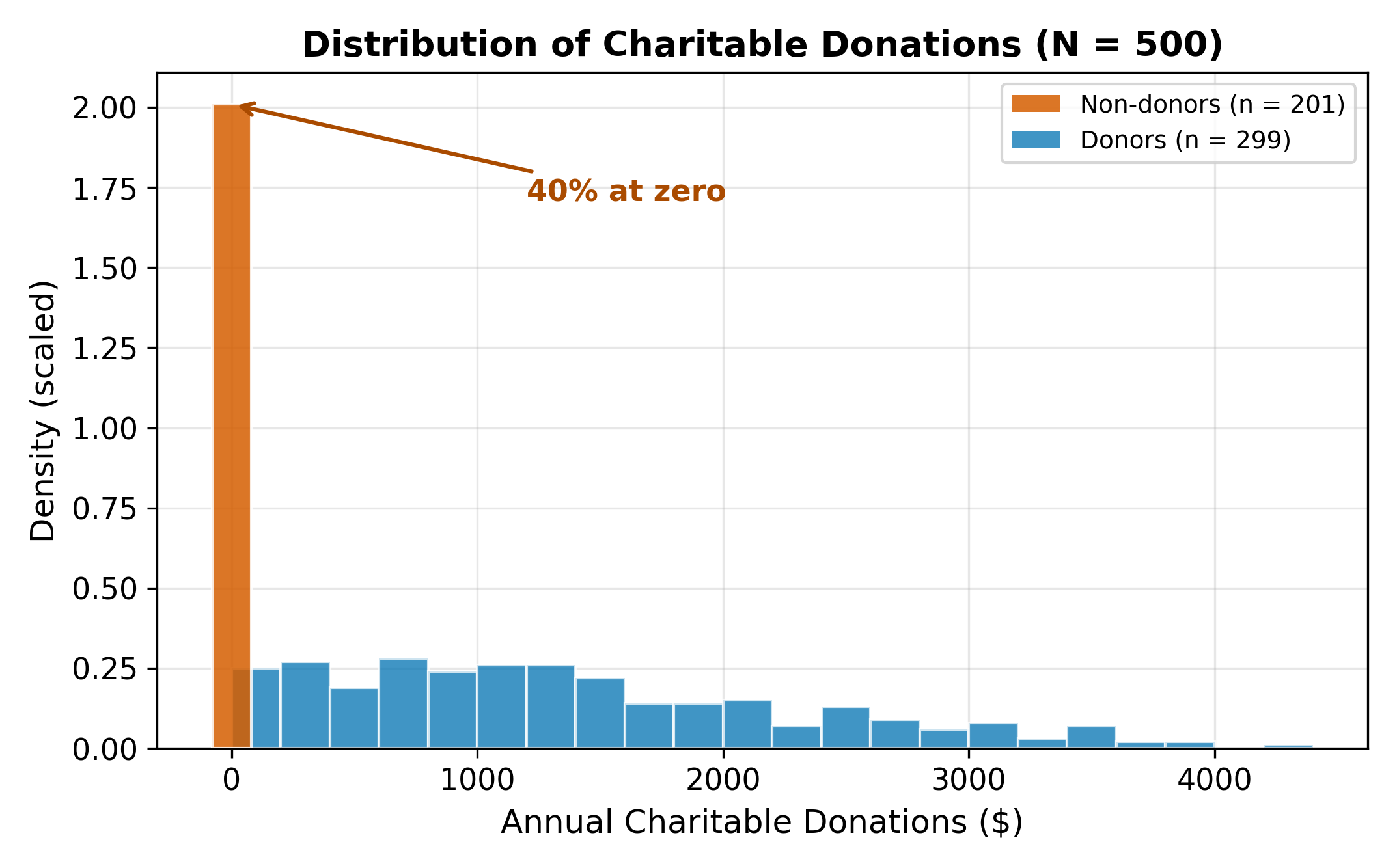
This pile-up at zero is not a data quality issue. It reflects a corner solution: many households evaluate the costs and benefits of donating and land at zero. They are not missing from the data. They genuinely chose not to give.
The same structure appears throughout economics:
- Hours of overtime are zero for workers who decline extra shifts
- Expenditure on luxury goods is zero for households that cannot afford them (or choose not to buy)
- Insurance claims are zero for policyholders who file no claims in a given year
- R&D spending is zero for firms that choose not to invest in research
\(\implies\) The dependent variable is continuous and positive for part of the sample, but piled up at a boundary for the rest. Standard regression tools are not designed for this.
19.2 Why OLS Fails
There are two natural OLS approaches, and both give biased estimates.
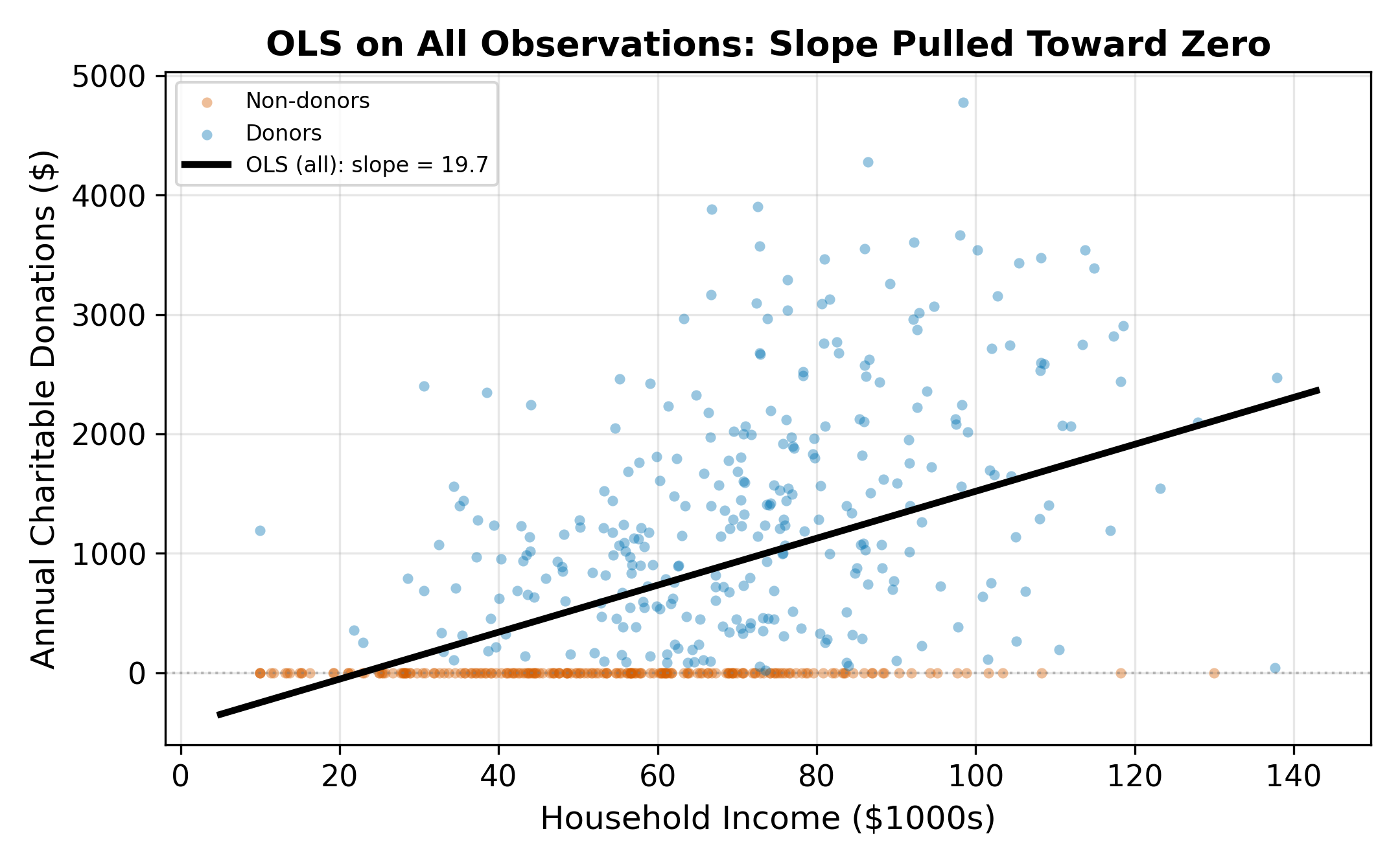
19.2.1 OLS on All Observations
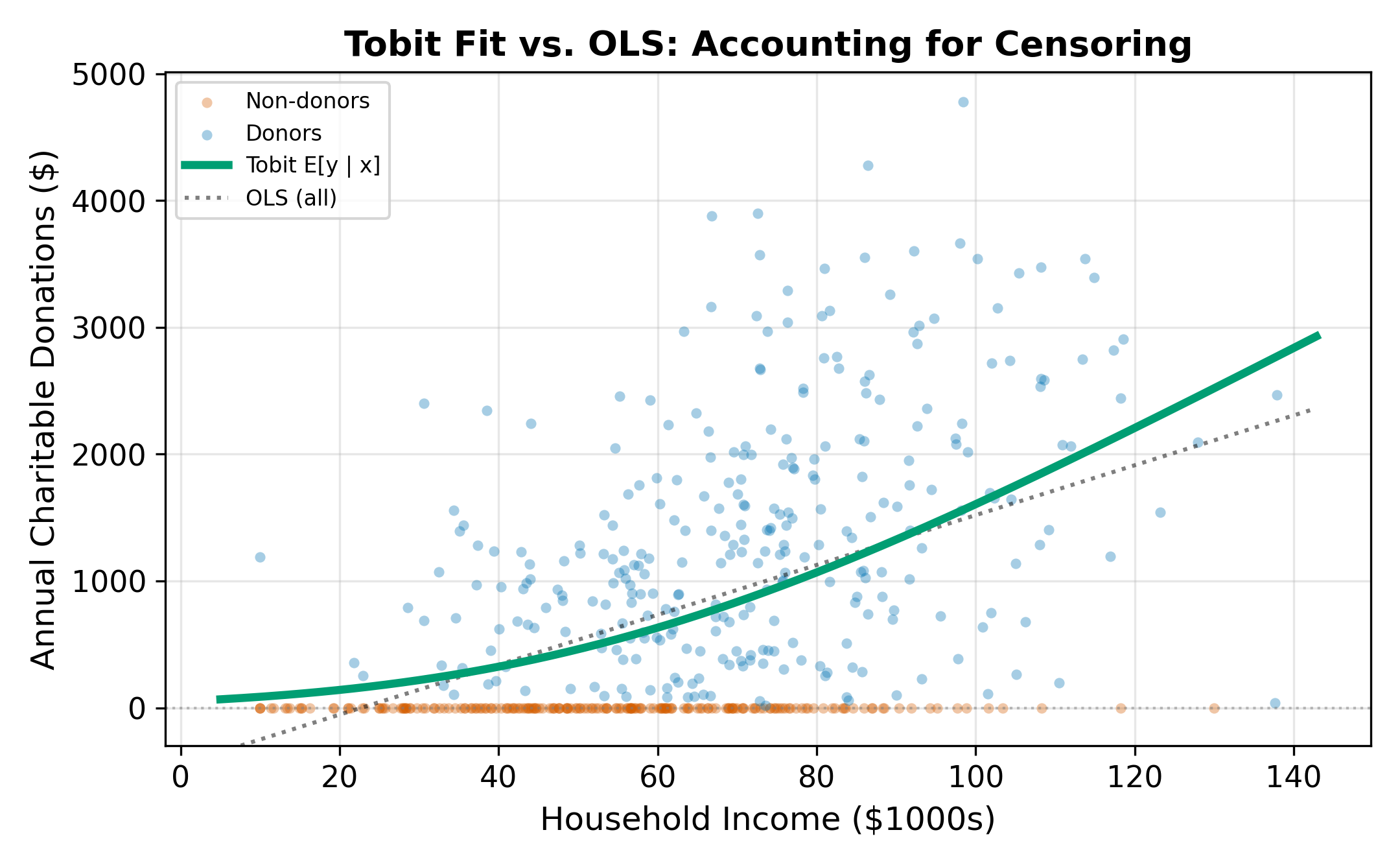
Running OLS on the full sample (including the zeros) forces the regression line to accommodate the mass at zero. The zeros pull the intercept down and flatten the slope. The resulting coefficient underestimates the true relationship between income and donations among people who do donate, and it misrepresents the process that generates the zeros.
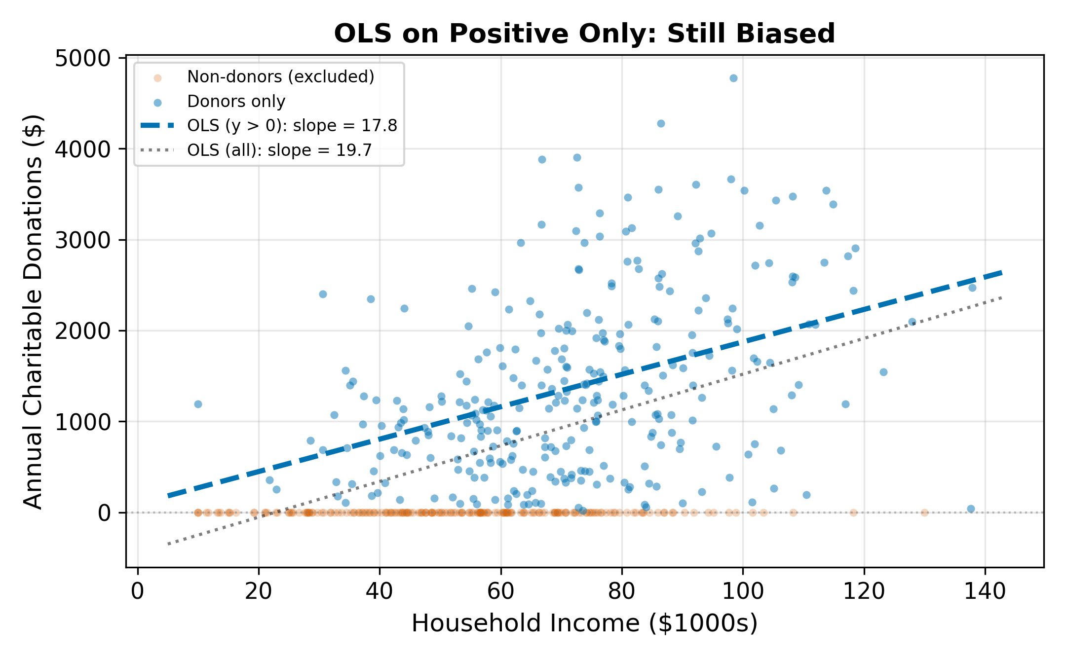
19.2.2 OLS on Positive Observations Only
Dropping the zeros and running OLS only on households that donated (\(y_i > 0\)) avoids the flattening problem but introduces a different bias: selection bias. The subsample of donors is not random. Higher-income, more-educated households are more likely to donate. By conditioning on \(y_i > 0\), we condition on the outcome, which distorts the relationship between the regressors and the donation amount.
To see why, note that among donors, the error term \(\varepsilon_i\) is not mean-zero. Conditioning on \(y_i > 0\) means conditioning on \(\varepsilon_i > -x_i'\beta\), which truncates the error distribution from below. The conditional expectation \(E[\varepsilon_i \mid \varepsilon_i > -x_i'\beta]\) is positive and varies with \(x_i\). This correlation between the (truncated) error and the regressors violates the OLS zero-conditional-mean assumption.
\(\implies\) Neither OLS approach works. Full-sample OLS underestimates the slope; positive-only OLS overestimates it by ignoring the selection process.
19.3 The Latent Variable Framework
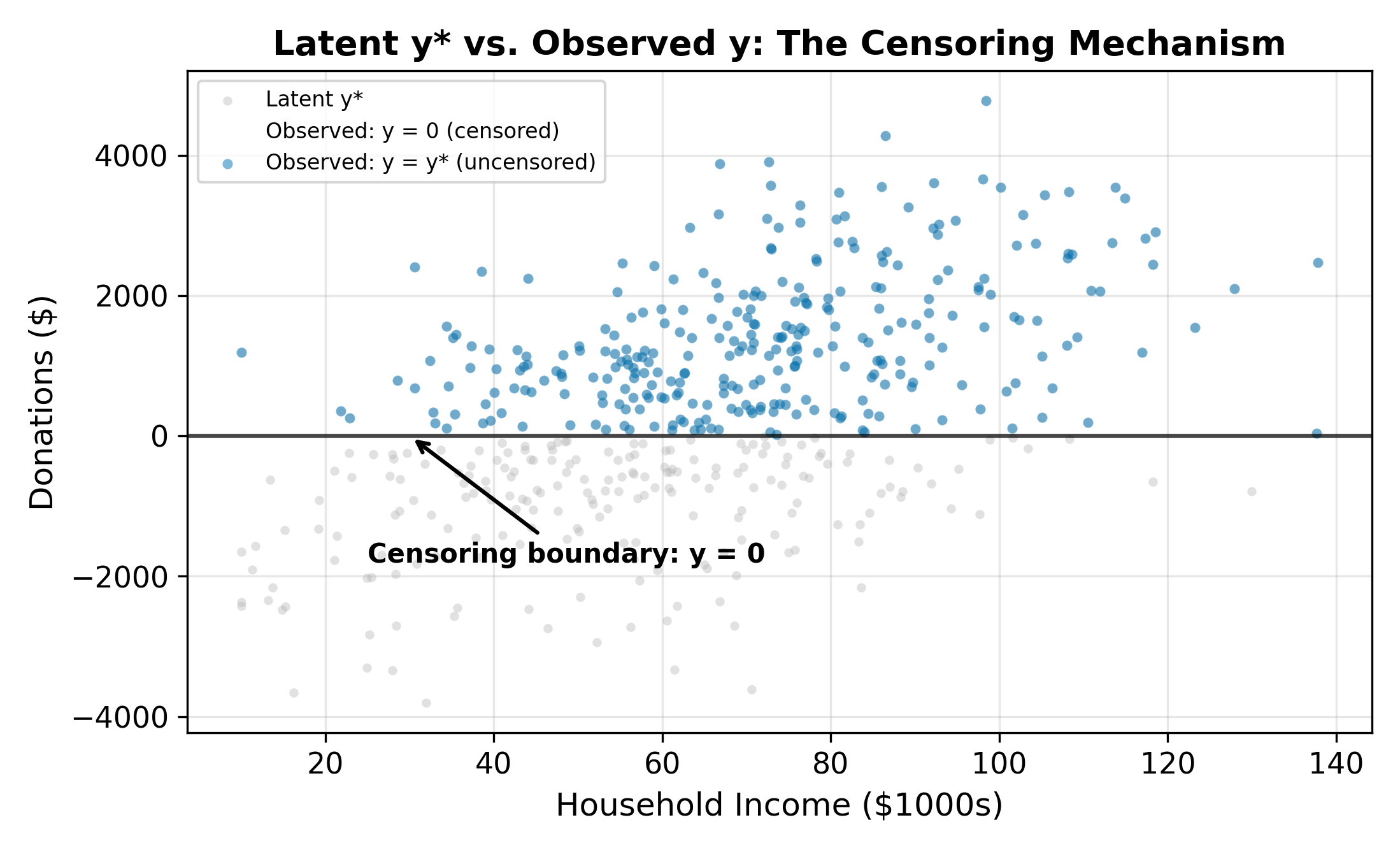
The Tobit model resolves both problems by positing a latent variable \(y_i^*\) that represents the household’s desired donation level. This latent variable can be negative (reflecting households whose characteristics point away from donating), but we never observe negative donations. Instead, the observed outcome is censored at zero.
The model:
\[ y_i^* = \beta_0 + \beta_1 \, \text{Income}_i + \beta_2 \, \text{Educ}_i + \beta_3 \, \text{Children}_i + \varepsilon_i, \quad \varepsilon_i \sim N(0, \sigma^2) \tag{19.1}\]
The censoring rule maps the latent variable to observed donations:
\[ y_i = \begin{cases} y_i^* & \text{if } y_i^* > 0 \\ 0 & \text{if } y_i^* \leq 0 \end{cases} \tag{19.2}\]
When \(y_i^* > 0\), we observe the actual latent value. When \(y_i^* \leq 0\), we observe only that the household chose not to donate. The zeros carry information (they tell us \(y_i^* \leq 0\)), but they don’t reveal how far below zero the latent variable fell.
The latent variable framework is the same one that generates probit and logit (from Binary Choice Models). The difference is that in binary choice, we only observe the sign of \(y^*\). In the Tobit model, we observe \(y^*\) itself whenever it is positive.
A negative \(y_i^*\) represents a household whose characteristics and idiosyncratic preferences point toward negative generosity. If donations could go below zero (i.e., if you could take money from charity), these households would. Since donations cannot be negative, they choose the corner solution: donate nothing. The more negative \(y_i^*\) is, the further the household is from the donation margin.
19.4 The Tobit Likelihood
Because the zeros and the positives are generated by different pieces of the latent variable distribution, the likelihood function has two components.
For positive observations (\(y_i > 0\)): We observe \(y_i = y_i^*\), so the contribution is the normal density evaluated at the observed value:
\[ f(y_i \mid x_i) = \frac{1}{\sigma} \phi\!\left(\frac{y_i - x_i'\beta}{\sigma}\right) \tag{19.3}\]
For zero observations (\(y_i = 0\)): We know only that \(y_i^* \leq 0\), which means \(\varepsilon_i \leq -x_i'\beta\). The contribution is the probability of this event:
\[ P(y_i = 0 \mid x_i) = \Phi\!\left(\frac{-x_i'\beta}{\sigma}\right) = 1 - \Phi\!\left(\frac{x_i'\beta}{\sigma}\right) \tag{19.4}\]
Combining both pieces, the log-likelihood is:
\[ \ln L = \sum_{y_i = 0} \ln\!\left[1 - \Phi\!\left(\frac{x_i'\beta}{\sigma}\right)\right] + \sum_{y_i > 0} \left[-\ln\sigma + \ln\phi\!\left(\frac{y_i - x_i'\beta}{\sigma}\right)\right] \tag{19.5}\]
MLE finds the \(\beta\) and \(\sigma\) that maximize Equation 19.5. The first sum captures the information in the zeros (how likely each zero is given the model); the second sum captures the information in the positive observations (how well the normal density fits the observed values).
Unlike OLS, the Tobit model estimates \(\sigma\) alongside \(\beta\). The scale of the error distribution matters because it determines how much of the latent variable distribution falls below zero. A larger \(\sigma\) means more censoring for any given \(x'\beta\).
19.5 Three Marginal Effects
In the Tobit model, a single coefficient \(\beta_k\) generates three distinct marginal effects, each answering a different question.
19.5.1 1. Effect on the Latent Variable \(E[y^*]\)
The simplest: \(\partial E[y^*] / \partial x_k = \beta_k\). This is the effect on desired donations, including the hypothetical negative values. Useful for understanding the underlying preference structure, but not directly observable.
19.5.2 2. Effect on the Probability of a Positive Outcome
A change in \(x_k\) shifts households across the zero boundary. The marginal effect on \(P(y > 0)\) is:
\[ \frac{\partial P(y_i > 0)}{\partial x_k} = \phi\!\left(\frac{x_i'\beta}{\sigma}\right) \cdot \frac{\beta_k}{\sigma} \tag{19.6}\]
This is the extensive margin: how does \(x_k\) affect the probability of donating at all? The \(\phi(\cdot)/\sigma\) factor ensures the effect is largest for households near the donation threshold and smallest for those deep in either tail.
19.5.3 3. Effect on the Unconditional Mean \(E[y]\)
The effect on expected donations (including the zeros) combines both margins:
\[ \frac{\partial E[y_i]}{\partial x_k} = \Phi\!\left(\frac{x_i'\beta}{\sigma}\right) \cdot \beta_k \tag{19.7}\]
This is the marginal effect most applied researchers report. It accounts for the fact that increasing income both makes donation more likely (extensive margin) and increases the amount given by those who already donate (intensive margin).
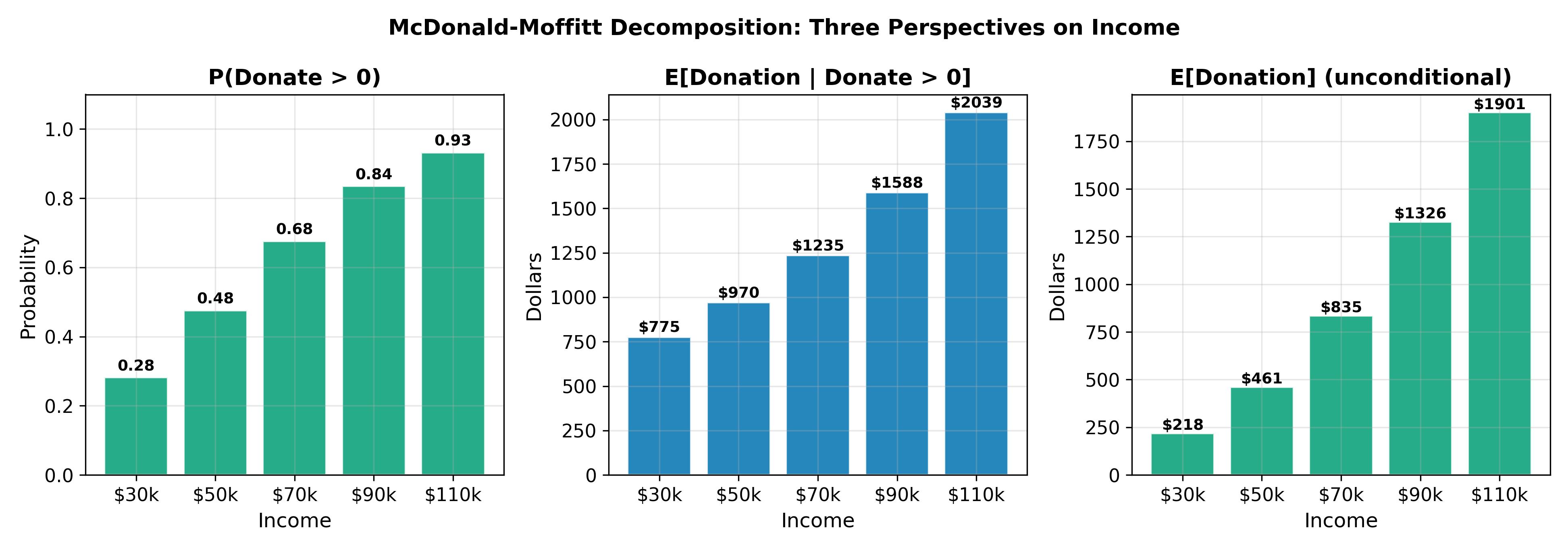
19.5.4 The McDonald-Moffitt Decomposition
McDonald and Moffitt (1980) formalized the decomposition of the unconditional marginal effect into its two components:
\[ \frac{\partial E[y]}{\partial x_k} = \underbrace{P(y > 0) \cdot \frac{\partial E[y \mid y > 0]}{\partial x_k}}_{\text{intensive margin}} + \underbrace{E[y \mid y > 0] \cdot \frac{\partial P(y > 0)}{\partial x_k}}_{\text{extensive margin}} \tag{19.8}\]
The intensive margin captures how much more existing donors give; the extensive margin captures how many new donors are brought in. This decomposition is valuable for policy analysis: a tax incentive for charitable giving might work primarily through one channel or the other.
The three marginal effects answer different questions. Always specify which one you are reporting: the effect on latent desired donations, the effect on the probability of donating, or the effect on expected donations including zeros.
The unconditional marginal effect \(\partial E[y] / \partial x_k\) is the right measure because it captures the total impact: both the increase in giving among current donors and the entry of new donors. But if the policymaker has a limited budget and must choose between programs that target potential donors (extensive margin) versus programs that encourage existing donors to give more (intensive margin), the McDonald-Moffitt decomposition reveals which channel is more responsive to each policy instrument.
19.6 Censoring vs. Truncation
The Tobit model applies to censored data. It is important to distinguish censoring from truncation, as they require different estimators.
| Censored | Truncated | |
|---|---|---|
| Definition | The dependent variable is capped at a boundary, but we observe all individuals | Observations below (or above) the boundary are excluded from the sample |
| Donation example | We survey all households; non-donors report \(y = 0\) | We survey only donors; non-donors are not in the data |
| What we know about zeros | We observe them (they are in the sample with \(y = 0\)) | We do not know they exist (sample contains only \(y > 0\)) |
| Information loss | Partial: we know \(y^* \leq 0\) but not the exact \(y^*\) | Complete: we do not observe the individual at all |
| Appropriate model | Tobit | Truncated regression |
| Sample size | Full population | Smaller (excludes zeros) |
A common source of confusion: if a survey is administered only to people who donated (truncation), the Tobit model is inappropriate. The likelihood in Equation 19.5 assumes we observe the zeros. With truncation, a truncated regression model is needed instead.
\(\implies\) Before estimating a Tobit, confirm that the zeros are observed in your data. If they are excluded by sample design, the data are truncated and require a different estimator.
This is truncation. People who had zero medical expenditures (they never visited the hospital) are absent from the data entirely. The researcher does not observe them and cannot include them in the estimation. The Tobit model would be inappropriate here because it assumes the zeros are in the sample. A truncated regression model or a two-part model that separately estimates hospital visit probability would be more appropriate.
19.7 Tobit Assumptions
The Tobit model relies on several assumptions, some testable and some not.
19.7.1 Normality
The latent errors \(\varepsilon_i\) are assumed \(N(0, \sigma^2)\). The likelihood function in Equation 19.5 is built entirely on the normal density and CDF. If the true error distribution is non-normal (e.g., heavy-tailed or skewed), the Tobit estimates are inconsistent.
This is a stronger requirement than for OLS, where non-normality affects inference but not consistency. In the Tobit model, the shape of the error distribution directly enters the likelihood through both the density \(\phi\) (for positive observations) and the CDF \(\Phi\) (for zeros). If the true errors are heavy-tailed, the model misjudges how many observations should be censored; if they are skewed, it misallocates probability mass between the two components.
Diagnostic checks include comparing the distribution of Tobit residuals (for positive observations) against the normal and examining whether predicted censoring rates match the observed share of zeros. Neither test is definitive, but large discrepancies signal misspecification.
19.7.2 Homoskedasticity
The error variance \(\sigma^2\) is assumed constant across observations. If \(\sigma^2\) varies with \(x\) (heteroskedastic Tobit), the standard model is misspecified: the estimated \(\sigma\) is a weighted average of the true variances, which distorts the likelihood and biases \(\hat{\beta}\). Extensions to heteroskedastic Tobit exist but are uncommon in applied work. In practice, grouping observations by a suspected source of heteroskedasticity and estimating separate Tobits can serve as an informal check.
19.7.3 The Single-Index Restriction
The most economically consequential assumption: the same parameter vector \(\beta\) governs both whether \(y^*\) crosses zero (the participation decision) and how large \(y^*\) is when it does (the amount decision). In the donations example, the single-index restriction says that the factors influencing whether you donate at all are the same factors (with the same relative weights) that determine how much you donate.
This is often unrealistic. The decision to donate at all may depend heavily on social pressure and religious affiliation, while the amount may depend primarily on income and wealth. When the participation and amount mechanisms differ, the Tobit model is misspecified.
Cragg’s double-hurdle model relaxes the single-index restriction by specifying separate equations for participation (a probit) and amount (a truncated regression). This allows different variables or different coefficients to govern the two decisions.
When the single-index assumption fails, the Heckman selection model provides an alternative that separates the participation equation from the outcome equation. See Heckman Selection for the full treatment.
\(\implies\) The Tobit model is appropriate when the same latent process generates both the zeros and the positive values. When participation and intensity are governed by different mechanisms, Heckman selection or the double-hurdle model is preferred.
Heckman Selection addresses the case where the single-index restriction fails: the participation decision and the outcome equation are governed by different processes. Return to the Qualitative and Limited DV hub for the full chapter map.