Show code
## Calculate Autocorrelations
den <- 333.8558
r1 <- 162.9753/den
r2 <- 112.4882/den
r3 <- 30.5802/den

## Calculate test statistics for significance
T <- 250
zc <- qnorm(0.975)/sqrt(T)Time Series: Stationarity, Autocorrelation, and Forecasting
These problems accompany Time Series. Read that chapter first for the theory behind these exercises.
Using 250 quarterly observations on U.S. GDP growth (G) from 1947Q2 to 2009Q3, we calculate the following quantities.
\[ \sum_t^{250} \left(G_t-\bar{G} \right)^2 = 333.8558 \hspace{0.5cm} \sum_t^{250} \left(G_t-\bar{G} \right)\left(G_{t-1}-\bar{G} \right) = 162.9753 \]
\[ \sum_t^{250} \left(G_t-\bar{G} \right)\left(G_{t-2}-\bar{G} \right) = 112.4882 \hspace{0.5cm} \sum_t^{250} \left(G_t-\bar{G} \right)\left(G_{t-3}-\bar{G} \right) = 30.5802 \]
Compute the first three autocorrelations \(r_1\), \(r_2\), and \(r_3\) for \(G\). Test whether each one is significantly different from zero at a \(5\%\) significance level. Sketch the first three bars of the correlogram. Include the significance bounds.
## Calculate Autocorrelations
den <- 333.8558
r1 <- 162.9753/den
r2 <- 112.4882/den
r3 <- 30.5802/den
## Calculate test statistics for significance
T <- 250
zc <- qnorm(0.975)/sqrt(T)The first three autocorrelations are
\(r_{1} =\) 0.4882
\(r_{2} =\) 0.3369
\(r_{3} =\) 0.0916
To test for significance, we use the null hypothesis that \(r_{k} = 0\) and the alternative of \(r_{k} \neq 0\) for \(k = 1,2,3\). Recall that our test statistic is of the form \(\hat{t}_{k} = \sqrt{T}\hat{r}_{k} \sim N(0,1)\). As such, for the test we will reject the null hypothesis for \(r_{k}\) if \(|r_{k}| >\) 0.124. Thus, we reject the null hypothesis that no autocorrelation exists at the one and two quarter horizon, and we fail to reject the null hypothesis that no autocorrelation exists at the three quarter horizon. This can be found in the following correlogram:
barplot(c(r1,r2,r3),xlab = "Lag",ylab = "Correlation", ylim = c(0,0.6),names.arg = c("1","2","3"))
abline(a = 0,b = 0)
abline(a = zc,b = 0)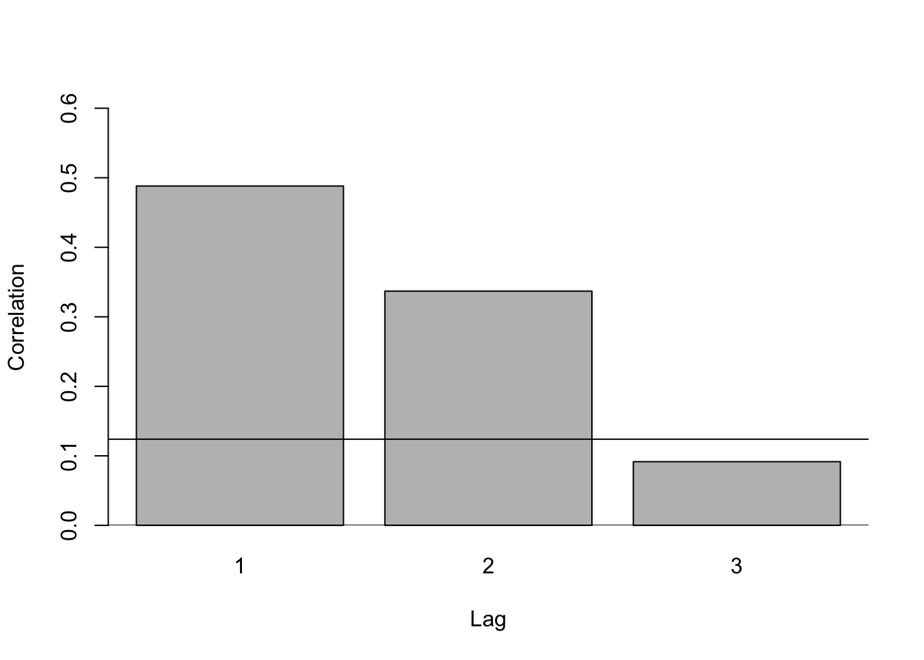
Given that \[\sum_t^{250} \left(G_t-\bar{G}_{-1} \right)^2 = 333.1119 \ \text{and} \ \sum_t^{250} \left(G_t-\bar{G}_{-1} \right)\left(G_t-\bar{G}_{1} \right) = 162.974\] where \[\bar{G}_{1}=\sum_{t=2}^{250} \frac{G_t}{249} = 1.662249 \ \text{and} \ \bar{G}_{-1}=\sum_{t=2}^{250} \frac{G_{t-1}}{249}= 1.664257,\] find the least squares estimate of \(\delta\) and \(\theta_1\) in the AR(1) model \(G_t = \delta + \theta_1 G_{t-1} + e_t\). Explain the difference between the estimate \(\theta_1\) and the estimate \(r_1\) obtained in part (a).
theta1 = 162.974/333.1119
delta = 1.662249 - theta1 * 1.664257
OLS estimates are \[ \hat{\theta}_{1} = \frac{\mathrm{Cov}(G_{t},G_{t - 1})}{\mathrm{Var}(G_{t})} = 0.4892 \] and \[ \hat{\delta} = \bar{G} - \hat{\theta}_{1}\bar{G}_{-1} = 0.8480 \] The estimated value of \(\hat{\theta}_{1}\) is slightly larger than the estimate for \(r_{1}\) because the summation in the denominator for \(r_{1}\) has one more squared term than the summation in the denominator for \(\hat{\theta}_{1}\). The calculated means are also slightly different.
Consider the infinite lag representation \(y_t = \alpha+\sum_{s=0}^{\infty}\beta_sx_{t-s} + e_t\) for the ARDL model \[y_t = \delta+\theta_1y_{t-1} + \theta_3y_{t - 3} + \delta_1x_{t-1} + v_t\]
Show that \(\alpha = \delta/(1-\theta_1-\theta_3), \beta_0=0,\beta_1=\delta_1,\beta_2=\theta_1\beta_1,\beta_3=\theta_1\beta_2,\beta_s=\theta_1\beta_{s-1}+\theta_3\beta_{s-3}\) for \(s \geq 4\)
Note that there are multiple ways to show this result. The method shown uses the lag operator \(L\).
Step 1: Rewrite the ARDL:
\[\begin{align*} y_{t} &= \delta + \theta_{1}y_{t - 1} + \theta_{3}y_{t - 3} + \delta_{1}x_{t - 1} + v_{t}\\ y_{t} &= \delta + L\theta_{1}y_{t} + L^{3}\theta_{3}y_{t} + L\delta_{1}x_{t} + v_{t}\\ y_{t} &= \delta + y_{t}(L\theta_{1} + L^{3}\theta_{3}) + L\delta_{1}x_{t} + v_{t}\\ y_{t} &= (1 - L\theta_{1} - L^{3}\theta_{3}) = \delta + L\delta_{1}x_{t} + v_{t}\\ y_{t} &= \frac{\delta}{1 - L\theta_{1}-L^{3}\theta_{3}} + \frac{L\delta_{1}}{1 - L\theta_{1}-L^{3}\theta_{3}}x_{t} + \eta_{t}\\ y_{t} &= \frac{\delta}{1 - L\theta_{1}-L^{3}\theta_{3}} + \frac{L\delta_{1}}{1 - L\theta_{1}-L^{3}\theta_{3}}x_{t} + \eta_{t} \end{align*}\]
Step 2: Rewrite the IDL:
\[\begin{align*} y_{t} = \alpha + \beta_{0}x_{t} + \beta_{1}x_{t - 1} + \beta_{2}x_{t-2} + \cdots + e_{t}\\ y_{t} = \alpha + L^{0}\beta_{0}x_{t} + L^{1}\beta_{1}x_{t} + L^{2}\beta_{2}x_{t} + \cdots + e_{t}\\ y_{t} = \alpha + \left(\sum_{s= 0}^{\infty}L^{s}\beta_{s}\right)x_{t} + e_{t} \end{align*}\]
Step 3: Combine the ARDL and IDL:
\[ \frac{\delta}{1 - L\theta_{1}-L^{3}\theta_{3}} + \frac{L\delta_{1}}{1 - L\theta_{1}-L^{3}\theta_{3}}x_{t} + \eta_{t} = \alpha + \left(\sum_{s= 0}^{\infty}L^{s}\beta_{s}\right)x_{t} + e_{t} \]
Matching “like” terms yields \[ \alpha = \frac{\delta}{1 - L\theta_{1} - L^{3}\theta_{3}} \implies \alpha = \frac{\delta}{1 - \theta_{1} - \theta_{3}} \] and
\[\begin{align*} \frac{L\delta_{1}}{1 - L\theta_{1} - L^{3}\theta_{3}} = &\sum_{s = 0}^{\infty}L^{s}\beta_{s}\\ L\delta_{1} = &(1 - L\theta_{1} - L^{3}\theta_{3})(L^{0}\beta_{0} + L^{1}\beta_{1} + L^{2}\beta_{2} + L^{3}\beta_{3} + \cdots)\\ L\delta_{1} = &L^{0}\beta_{0} - L^{1}\theta_{1}\beta_{0} - L^{3}\theta_{3}\beta_{0} + \\ &L^{1}\beta_{1} - L^{2}\theta_{1}\beta_{1} - L^{4}\theta_{3}\beta_{1} + \\ &L^{2}\beta_{2} - L^{3}\theta_{1}\beta_{2} - L^{5}\theta_{3}\beta_{2} + \\ &L^{3}\beta_{3} - L^{4}\theta_{1}\beta_{3} - L^{5}\theta_{3}\beta_{2} + \cdots \end{align*}\]
Grouping by the lag terms (L’s) yields \[ L\delta_{1} = L^{0}\beta_{0} + L^{1}(\beta_{1} - \theta_{1}\beta_{0}) + L^{2}(\beta_{2} - \theta_{1}\beta_{1}) + L^{3}(\beta_{3} - \theta_{1}\beta_{2} - \theta_{3}\beta_{0}) + L^{4}(\beta_{4} - \theta_{1}\beta_{3} - \theta_{3}\beta_{1}) + \cdots \]
Suppose the left side was written like this: \[ L^{0}(0) + L^{1}\delta_{1} + L^{2}(0) + L^{3}(0) + L^{4}(0) + \cdots \]
Then connecting the two sides of the equation yields:
\[\begin{align*} \beta_{0} &= 0\\ \beta_{1} &= \delta_{1} + \theta_{1}\beta_{0} = \delta_{1}\\ \beta_{2} &= \theta_{1}\beta_{1}\\ \beta_{3} &= \theta_{1}\beta_{2} + \theta_{3}\beta_{0} = \theta_{1}\beta_{2}\\ \beta_{4} &= \theta_{1}\beta_{3} + \theta_{3}\beta_{1}\\ \beta_{s} &= \theta_{1}\beta_{s - 1} + \theta_{3}\beta_{s - 3} \end{align*}\]
Using quarterly data on U.S. inflation (INF), and the change in the unemployment rate (DU) from 1955Q2 to 2016Q1, we estimate the following version of a Phillips curve
\[ \begin{array}{l l l l l} \hat{INF}_{t} =& 0.094 + & 0.564INF_{t - 1} +& 0.333INF_{t - 3} - & 0.300DU_{t -1}\\ \text{(se)} & (0.049) & (0.051) & (0.052) & (0.0084) \end{array} \qquad \qquad SSE = 48.857 \]
Using the results in part (a), find estimates of the first 12 lag weights in the infinite lag representation of the estimated Phillips curve in part (b). Graph those weights and comment on the graph.
## Calculate lags of betas using information from (a) and (b)
Beta_0 <- 0
Beta_1 <- -0.3
Beta_2 <- 0.564 * Beta_1
Beta_3 <- 0.564 * Beta_2
Beta_4 <- 0.564 * Beta_3 + 0.333*Beta_1
Beta_5 <- 0.564 * Beta_4 + 0.333*Beta_2
Beta_6 <- 0.564 * Beta_5 + 0.333*Beta_3
Beta_7 <- 0.564 * Beta_6 + 0.333*Beta_4
Beta_8 <- 0.564 * Beta_7 + 0.333*Beta_5
Beta_9 <- 0.564 * Beta_8 + 0.333*Beta_6
Beta_10 <- 0.564 * Beta_9 + 0.333*Beta_7
Beta_11 <- 0.564 * Beta_10 + 0.333*Beta_8
Beta_12 <- 0.564 * Beta_11 + 0.333*Beta_9

## Set up a dataframe for later plotting
betas <- data.frame(c(Beta_0,Beta_1,Beta_2,Beta_3,Beta_4,Beta_5,Beta_6,
                      Beta_7,Beta_8,Beta_9,Beta_10,Beta_11,Beta_12))
betas$ID <- seq.int(nrow(betas)) - 1
names(betas) <- c("Betas","Lags")

## Use ggplot to graph
ggplot(data = betas, aes(x = Lags, y = Betas)) +
       geom_point(color = "lightblue", size = 3) +
       geom_line() +
       labs(title = "Lags of betas") +
       theme_minimal()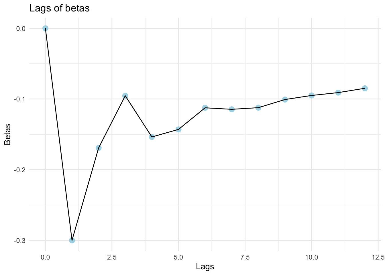
What rate of inflation is consistent with a constant unemployment rate (where DU = 0 in all time periods)?
A constant rate of inflation is one where \(INF_{t} = INF_{t - s} = INF\) for all periods \(t\) and lags \(s\). With \(DU = 0\), the model becomes:
\[ INF = 0.094 + 0.564INF + 0.333INF \implies INF = \frac{0.094}{1 - 0.564 - 0.333} \]
INF <- 0.094/(1 - 0.564 - 0.333)We find that the constant rate of inflation is 0.9126.
Let \(\hat{e}_t = 0.564 \hat{e}_{t-1} + 0.33 \hat{e}_{t-3} + \hat{u}_t\) where the \(\hat{u}_t\) are the residuals from the equation in part (b), and the initial values \(\hat{e}_1\), \(\hat{e}_2\), and \(\hat{e}_3\) are set equal to zero. The SSE from regressing \(\hat{u}_t\) on a constant, \(INF_{t-1},INF_{t-3},DU_{t-1}, \hat{e}_{t-1}\), and \(\hat{e}_{t-3}\) is 47.619. Using a \(5\%\) significance level, test the hypothesis that the errors in the infinite lag representation follow the AR(3) process \(e_t = \theta_1e_{t-1} + \theta_3e_{t-3} + v_t\). The number of observations used in this regression and that in part (b) is 241. What are the implications of this test result?
R2 <-  1 - 47.619/48.857
LM <- 241 * R2
qchi <- qchisq(0.95, 2)
Recall that the LM style test uses the \(N\times R^{2}\) test statistic. To calculate the \(R^{2}\) of this regression, we want to follow the formula \(R^{2} = 1 - \frac{SSE}{SST}\). As our “\(Y\)” variable is the errors from part (b), the \(SST\) will be given by the \(SSE\) from that regression: \(SST = 48.857\). With the SSE of this LM regression, we calculate the \(R^{2}\) as
\[ R^{2} = 1 - \frac{SSE}{SST} = 1 - \frac{47.619}{48.857} = 0.0253 \]
The LM test statistic is then given by \(N \times R^{2} = 6.1068\), which is greater than our chi-squared critical value of 5.9915. This indicates that the errors do not follow an AR(3) process.
In Examples 9.14 and 9.15, we considered the Phillips curve \(INF_t = INF_t^E - \gamma \left(U_t - U_{t-1} \right) + e_t = \alpha + \beta_0 DU_t + e_t\) where inflationary expectations are assumed to be constant, \(INF_t^E = \alpha\), and \(\beta_0=-\gamma\). In Example 9.15, we used data in the file phillips5_aus to estimate this model assuming the errors follow an AR(1) model \(e_t =\rho e_{t-1}\). Nonlinear least squares estimates of the model were \(\hat{\alpha} = 0.7028\), \(\hat{\beta}_0 = -0.3830\), and \(\hat{\rho}=0.5001\). The equation from these estimates can be written as the following ARDL representation:
\[\begin{align*} \hat{INF}_{t} &= \hat{\alpha}(1 - \hat{\rho}) + \hat{\rho}INF_{t - 1} + \hat{\beta}_{0}DU_{t} - \hat{\rho}\hat{\beta}_{0}DU_{t - 1}\\ &= 0.7028 \times (1 - 0.5001) + 0.5001INF_{t - 1} - 0.3830DU_{t} + (0.50001 \times 0.3830) DU_{t - 1}\\ &= 0.3513 + 0.5001INF_{t - 1} - 0.3830 DU_{t} + 0.1915 DU_{t - 1} \tag{XR 9.21.1} \end{align*}\]
Instead of assuming that this ARDL(1, 1) model is a consequence of an AR(1) error, another possible interpretation is that inflationary expectations depend on actual inflation in the previous quarter, \(INF_t^E = \delta + \theta_1 INF_{t-1}\). If \(DU_{t-1}\) is retained because of a possible lagged effect, and we change notation so that it is in line with what we are using for a general ARDL model, we have the equation:
\[ INF_t =\delta + \theta INF_{t-1} + \delta_0 DU_t + \delta_1 DU_{t-1} + e_t \tag{XR 9.21.2}\]
Find least squares estimates of the coefficients in \((XR \ \ 9.21.2)\) and compare these values with those in \((XR \ \ 9.21.1)\). Use HAC standard errors.
# Load in dataset and convert to time series
phillips_df <- read.csv('data/phillips5_aus.csv')
phillips_df.ts <- ts(phillips_df,
                     start = c(1987,1),
                     end = c(2016,1),
                     frequency = 4)

# estimate model 9.21.2
reg.mod <- dynlm(inf~L(inf, 1) + du + L(du, 1), data=phillips_df.ts)

# obtain HAC SE using NeweyWest function from sandwich package
reg.modHAC <- coeftest(reg.mod, vcov.= NeweyWest(reg.mod))
tidy(reg.modHAC) %>% kable()| term | estimate | std.error | statistic | p.value |
|---|---|---|---|---|
| (Intercept) | 0.3483 | 0.0987 | 3.5300 | 0.0006 |
| L(inf, 1) | 0.4992 | 0.1284 | 3.8890 | 0.0002 |
| du | -0.3728 | 0.1464 | -2.5462 | 0.0122 |
| L(du, 1) | 0.0171 | 0.1503 | 0.1141 | 0.9094 |
Reestimate \((XR \ \ 9.21.2)\) after dropping \(DU_{t-1}\). Why is it reasonable to drop \(DU_{t-1}\)?
It is reasonable to drop \(DU_{t - 1}\) because the \(p\)-value for its estimated coefficient is significantly different from zero.
# estimate model 9.21.2
reg.mod_noDU <- dynlm(inf~L(inf, 1) + du, data=phillips_df.ts)

# obtain HAC SE using NeweyWest function from sandwich package
reg.modHAC_noDU <- coeftest(reg.mod, vcov.= NeweyWest(reg.mod_noDU))
tidy(reg.modHAC_noDU) %>% kable()| term | estimate | std.error | statistic | p.value |
|---|---|---|---|---|
| (Intercept) | 0.3483 | 0.0986 | 3.532 | 0.0006 |
| L(inf, 1) | 0.4992 | 0.1270 | 3.931 | 0.0001 |
| du | -0.3728 | 0.1388 | -2.686 | 0.0083 |
Now, suppose that inflationary expectations depend on inflation in the previous quarter and inflation in the same quarter last year, \(INF_t^E = \delta + \theta_1 INF_{t-1} +\theta_4 INF_{t-4}\). Estimate the model that corresponds to this assumption.
Now our model is given by
\[ INF_{t} = INF_{t}^{E} - \gamma (U_{t} - U_{t - 1}) + e_{t} = \delta + \theta_{1} INF_{t - 1} + \theta_{4} INF_{t - 4} + \delta_{0}DU_{t} + e_{t} \]
# estimate the new model with this four-period lagged term
reg.mod_l4 <- dynlm(inf~L(inf, 1) + L(inf, 4) + du, data=phillips_df.ts)
# get HAC SE
reg.mod_l4HAC <- coeftest(reg.mod_l4, vcov.=NeweyWest(reg.mod_l4))
tidy(reg.mod_l4HAC) %>% kable()| term | estimate | std.error | statistic | p.value |
|---|---|---|---|---|
| (Intercept) | 0.1722 | 0.0736 | 2.339 | 0.0212 |
| L(inf, 1) | 0.3282 | 0.0996 | 3.295 | 0.0013 |
| L(inf, 4) | 0.3789 | 0.0701 | 5.406 | 0.0000 |
| du | -0.5653 | 0.1200 | -4.712 | 0.0000 |
Is there empirical evidence to support the model in part (c)? In your answer, consider (i) the residual correlograms from the equations estimated in parts (b) and (c), and the significance of coefficients in the complete ARDL(4, 0) model that includes \(INF_{t-2}\) and \(INF_{t-3}\).
In our model for part (c), our estimate of the coefficient on the fourth lag has a \(p\)-value much smaller than \(5\%\), which gives evidence that the lag should be included. Let’s also look at the correlograms for both models:
# we will use the tseries package to generate a correlogram of the residuals
# model (b), where we did not have the DUt-4 term
residb_ts = ts(resid(reg.mod_noDU))
acf(residb_ts, main = "Model (b) Residuals")
# model (c), where we did have the DUt-4 term
residc_ts = ts(resid(reg.mod_l4))
acf(residc_ts, main = "Model (c) Residuals")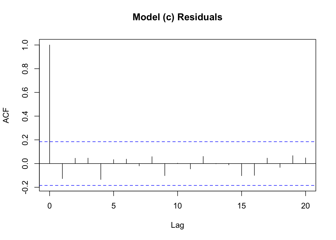
In part (b) when we don’t have the 4-quarter lag within the estimated model, we notice a spike in the correlogram at that fourth lag. This indicates that there is some issue with our choice of included lags in part (b). In part (c) after we introduce the fourth lag, this spike disappears. This further supports that the 4-quarter lag should be included in the model.
Reconsider the data file
inequalityused in Exercise 9.26 and the model in part (a) of that exercise but include the median marginal tax rate for the upper 1% of incomes (\(TAX\)). We are interested in whether the marginal tax rate is a useful instrument for reducing inequality. The resulting model is\[ SHARE_{t} = \alpha_{1} + \alpha_{2}TAX_{t} + \alpha_{3}YEAR_{t} + \alpha_{4}YEAR_{t}^{2} + e_{t} \]
Estimate the equation using data for Canada. Obtain both conventional and HAC standard errors. Compare the 95% interval estimate for \(\alpha_{2}\) for each of the standard errors.
# Read in the data file from CSV
inequality = read.csv('data/inequality.csv')

# Alternatively, load the data from the POE5Data library with

### inequality = data(inequality)

inequality = ts(
    data = inequality,
    start = 1,
    end = 80,
    frequency = 1
)

# Estimate the linear model (this model has conventional OLS standard errors)
lm.model.27a = dynlm(data = inequality, formula = ca_share ~ ca_tax + year + I(year^2))

# Compute the HAC standard errors
HAC.27a = coeftest(lm.model.27a, vcov = NeweyWest)

# Construct interval estimates of the two
crit = qt(0.975, 76)
a2 = lm.model.27a$coefficients[2]

margin.OLS = crit * coeftest(lm.model.27a)[6]
CI.OLS = c(a2 - margin.OLS, a2 + margin.OLS)

margin.HAC = crit * HAC.27a[6]
CI.HAC = c(a2 - margin.HAC, a2 + margin.HAC)
The estimated model and both standard errors are given by:
| Estimate | OLS SE | HAC SE | |
|---|---|---|---|
| (Intercept) | 17.8080 | 0.4751 | 2.6162 |
| ca_tax | -0.1069 | 0.0177 | 0.0638 |
| year | -0.1741 | 0.0395 | 0.1320 |
| I(year^2) | 0.0019 | 0.0004 | 0.0012 |
The confidence interval for \(\alpha_{2}\) computed using OLS standard errors is \([-0.1422, -0.0715]\). The confidence interval for \(\alpha_{2}\) computed using the HAC standard errors is \([-0.2339, 0.0202]\). The HAC interval is noticeably wider than the OLS interval, which indicates that autocorrelated errors might be making the OLS standard errors incorrect.
Use an LM test with a 5% significance level and three lagged residuals to test for autocorrelation in the errors of the equation estimated in part (a). What do you conclude about the use of HAC standard errors in part (a)?
bgtest(lm.model.27a, order = 3, fill = 0)
    Breusch-Godfrey test for serial correlation of order up to 3

data:  lm.model.27a
LM test = 57, df = 3, p-value = 3e-12
As the p-value is significantly smaller than the \(5\%\) significance level, we can conclude that the errors are serially correlated. The use of HAC standard errors in part (a) is justified.
Estimate a parameter \(\rho\) by applying OLS to the equation \(\hat{e}_{t} = \rho \hat{e}_{t - 1} + \hat{v}_{t}\) where \(\hat{e}_{t}\) are the least squares residuals from part (a). What assumption is being made when you estimate the equation?
resid = resid(lm.model.27a)
lm.model.27c = dynlm(resid~L(resid))
rhohat = lm.model.27c$coefficients[2]
We obtain \(\hat{\rho} = 0.8482\). The critical assumption we are making is that the \(v\)’s are not autocorrelated.
Transform each of the variables in the original equation using a transformation of the form \(x_{t}^{*} = x_{t} - \hat{\rho}x_{t - 1}\) and apply OLS to the transformed variables. Compute both conventional and HAC standard errors. Find the resulting \(95\%\) interval estimates for \(\alpha_{2}\). Compare them with each other and those found in part (a).
# Create adjusted versions of the variables and group them into a single time series object
lag <- stats::lag
inequality_adj <-cbind(inequality[,"ca_share"] - rhohat*lag(inequality[,"ca_share"],-1),
                       inequality[,"ca_tax"] - rhohat*lag(inequality[,"ca_tax"],-1),
                       inequality[,"year"] - rhohat*lag(inequality[,"year"],-1),
                       inequality[,"year"]^2 - rhohat*lag(inequality[,"year"],-1)^2)
colnames(inequality_adj) <- c("ca_share_adj","ca_tax_adj","year_adj","year2_adj")


# Repeat steps from part A

# Estimate the linear model (this model has conventional OLS standard errors)
lm.model.27d = dynlm(data = inequality_adj,
                     formula = ca_share_adj ~ ca_tax_adj + year_adj + year2_adj)

# Compute the HAC standard errors
HAC.27d = coeftest(lm.model.27d, vcov = NeweyWest)

# Construct interval estimates of the two
crit = qt(0.975, 76)
a2 = lm.model.27d$coefficients[2]

margin.OLS = crit * coeftest(lm.model.27d)[6]
CI.OLS = c(a2 - margin.OLS, a2 + margin.OLS)

margin.HAC = crit * HAC.27d[6]
CI.HAC = c(a2 - margin.HAC, a2 + margin.HAC)
The estimated model and both standard errors are given by:
| Estimate | OLS SE | HAC SE | |
|---|---|---|---|
| (Intercept) | 2.9821 | 0.3296 | 0.4209 |
| ca_tax_adj | -0.0411 | 0.0163 | 0.0184 |
| year_adj | -0.3684 | 0.1088 | 0.1187 |
| year2_adj | 0.0037 | 0.0011 | 0.0012 |
The confidence interval for \(\alpha_{2}\) computed using OLS standard errors is \([-0.0735, -0.0086]\). The confidence interval for \(\alpha_{2}\) computed using the HAC standard errors is \([-0.0777, -0.0044]\). Because the two standard errors are similar, the two intervals are approximately the same. This suggests that the GLS estimation method has eliminated the autocorrelation. They are very different from the intervals in part (a), largely because the estimate of \(\hat{\alpha}_{2}\) has changed considerably.
Use an LM test with a \(5\%\) significance level and three lagged residuals to test for autocorrelation in the errors of the equation estimated in part (d). What do you conclude about the use of HAC standard errors in part (d)?
bgtest(lm.model.27d, order = 3, fill = 0)
    Breusch-Godfrey test for serial correlation of order up to 3

data:  lm.model.27d
LM test = 6.6, df = 3, p-value = 0.08
As the p-value is larger than the \(5\%\) significance level, we cannot conclude that the errors are autocorrelated in the GLS model. The HAC errors are not required for the model of part (d).
For each of the equations estimated in part (a) and (d), discuss whether the exogeneity assumption required for consistent estimation of \(\alpha_{2}\) is likely to be satisfied.
The exogeneity condition requires the variable \(TAX_{t}\) to be uncorrelated with any omitted variables whose effects are also included in the error term. In this example, this condition is unlikely to be satisfied. For example, both the income share of the top 1% of earners and the tax they pay might be correlated with the growth rate of the economy, whose impact will be felt in the error term. For OLS to be consistent \(e_{t}\) must be uncorrelated with current and past values of \(TAX\). For GLS to be consistent, \(e_{t}\) must instead be uncorrelated with the future value \(TAX_{t + 1}\), as well as current and past values. In other words, if \(TAX\) is correlated with the growth rate in the previous period, then GLS will be inconsistent. This additional condition is the likely cause of the discrepancy in the OLS and GLS estimates for \(\alpha_{2}\).
In this exercise, we consider a partial adjustment model as an alternative to the model used in Exercise 9.29 for modeling sugar cane area response in Bangladesh. The data are in the file
bangla5. In the partial adjustment model, long-run desired area, \(AREA^{*}\) is a function of price,\[ AREA_{t}^{*} = \alpha + \beta_{0}PRICE_{t} \tag{XR 9.30.1} \]
In the short-run, fixed resource constraints prevent farmers from fully adjusting to the area desired at the prevailing price. Specifically,
\[ AREA_{t} - AREA_{t - 1} = \gamma(AREA_{t}^{*} - AREA_{t-1}) + e_{t} \tag{XR 9.30.2} \]
where \(AREA_{t} - AREA_{t - 1}\) is the actual adjustment from the previous year, \(AREA_{t}^{*} - AREA_{t - 1}\) is the desired adjustment for the previous year, and \(0 < \gamma < 1\).
Combine (XR 9.30.1) and (XR 9.30.2) to show that an estimable form of the model can be written as
\[ AREA_{t} = \delta + \theta_{1} AREA_{t - 1} + \delta_{0}PRICE_{t} + e_{t} \]
where \(\delta = \alpha\gamma\), \(\theta_{1} = 1 - \gamma\), and \(\delta_{0} = \beta_{0}\gamma\).
Beginning with (XR 9.30.2), we substitute (XR 9.30.1) into the equation for \(AREA_{t}^{*}\) and move \(AREA_{t - 1}\) to the right hand side:
\[ AREA_{t} = AREA_{t - 1} + \gamma(\alpha + \beta_{0}PRICE_{t} - AREA_{t - 1}) + e_{t} \]
Next, simplify the equation and group like variables:
\[ AREA_{t} = \underbrace{\gamma\alpha}_\delta + \underbrace{(1 - \gamma)}_{\theta_{1}}AREA_{t -1} + \underbrace{\gamma\beta_{0}}_{\delta_{0}}PRICE_{t} + e_{t} \]
Find least squares estimates of \(\delta\), \(\theta_{1}\), and \(\delta_{0}\). Are they significantly different from zero at a \(5\%\) significance level?
# Load data and convert it to a time series object
bangla5 <- read.csv("data/bangla5.csv")
bangla.ts <- ts(bangla5)

# Compute the OLS estimates for the problem
reg.bangla <- dynlm(area ~ L(area,1) + price, data = bangla.ts)
print(summary(reg.bangla))
Time series regression with "ts" data:
Start = 2, End = 73

Call:
dynlm(formula = area ~ L(area, 1) + price, data = bangla.ts)

Residuals:
   Min     1Q Median     3Q    Max
 -41.4  -15.6    0.3   17.9   47.9

Coefficients:
            Estimate Std. Error t value Pr(>|t|)
(Intercept) -41.2753    13.8124   -2.99   0.0039 **
L(area, 1)    0.5237     0.0814    6.43  1.4e-08 ***
price        64.0614    11.1801    5.73  2.4e-07 ***
---
Signif. codes:  0 '***' 0.001 '**' 0.01 '*' 0.05 '.' 0.1 ' ' 1

Residual standard error: 21 on 69 degrees of freedom
Multiple R-squared:  0.556, Adjusted R-squared:  0.543
F-statistic: 43.1 on 2 and 69 DF,  p-value: 7.09e-13
The p-values indicate that all three coefficients are significant.
What are the first three autocorrelations of the residuals? Are they significantly different from zero at a \(5\%\) significance level?
# Pull the residuals from the model, compute the autocorrelations, and find the critical level
resid.bangla = resid(reg.bangla)
ac.bangla = acf(resid.bangla,pl = FALSE)
cR = 1.96/sqrt(73)
The first three residual autocorrelations are \(r_{1} = 0.0146\), \(r_{2} =0.0451\), and \(r_{3} = 0.1673\). All of the residuals fall within the critical value of \(\pm0.2294\), so none are significantly different from zero at the \(5\%\) level.
Find estimates and standard errors for \(\alpha\), \(\beta_{0}\), and \(\gamma\). Are the estimates significantly different from zero at a \(5\%\) significance level?
We can compute the original parameters from the model in (a) in the following way:
For the standard errors, we have \(se(\gamma) = se(\theta_{1})\), but the delta rule will be used to compute the standard errors of the other two. For a function with two variables \(y = f(x,z)\), the Delta Method states:
\[ \mathrm{Var}(y) = \left(\frac{\partial y}{\partial x}\right)^{2}\mathrm{Var}(x) + \left(\frac{\partial y}{\partial z}\right)^{2}\mathrm{Var}(z) + 2\left(\frac{\partial y}{\partial x}\right)\left(\frac{\partial y}{\partial z}\right)\mathrm{Cov}(x,z) \]
In our example, we have \(f(x,z) = \frac{x}{1 - z}\), with \(\alpha = f(\delta,\theta_{1})\) and \(\beta_{0} = f(\delta_{0},\theta_{1})\). This yields:
\[\frac{\partial y}{\partial x} = \frac{1}{1 - z} \ \ \text{and} \ \ \frac{\partial y}{\partial z} = \frac{x}{(1 - z)^{2}}\]
Thus, the variance for \(\alpha\) and \(\beta\) will be computed with the following formulas:
\[\begin{align*} \mathrm{Var}(\alpha) &= \left(\frac{1}{1 - \theta_{1}}\right)^{2}\mathrm{Var}(\delta) + \left(\frac{\delta}{(1 - \theta_{1})^{2}}\right)^{2}\mathrm{Var}(\theta_{1}) + 2\left(\frac{1}{1 - \theta_{1}}\right)\left(\frac{\delta}{(1 - \theta_{1})^{2}}\right)\mathrm{Cov}(\delta,\theta_{1})\\ \mathrm{Var}(\beta_{0}) &= \left(\frac{1}{1 - \theta_{1}}\right)^{2}\mathrm{Var}(\delta_{0}) + \left(\frac{\delta_{0}}{(1 - \theta_{1})^{2}}\right)^{2}\mathrm{Var}(\theta_{1}) + 2\left(\frac{1}{1 - \theta_{1}}\right)\left(\frac{\delta_{0}}{(1 - \theta_{1})^{2}}\right)\mathrm{Cov}(\delta_{0},\theta_{1}) \end{align*}\]
The standard errors are computed as the square root of these variances, with hypothesis tests following from them as usual:
# Pull coefficients and the covariance matrix
del <- reg.bangla$coefficients[[1]]
theta1 <- reg.bangla$coefficients[[2]]
del0 <- reg.bangla$coefficients[[3]]
Cov <- vcov(reg.bangla)

# Calculate the original parameter estimates
gamma <- 1 - theta1
alpha <- del/gamma
beta <- del0/gamma

# Calculate the SE for gamma and conduct the test
var_g = Cov[2,2]
SE_g = sqrt(var_g)
tg = gamma/SE_g
g = c(gamma, SE_g, tg)

# Calculate the SE for alpha and conduct the test
part_del = (1/gamma)
part_theta1 = (del/(1 - theta1)^2)
var_a = Cov[1,1]*part_del^2 + Cov[2,2]*part_theta1^2 + 2*part_del*part_theta1*Cov[1,2]
SE_a = sqrt(var_a)
ta = alpha/SE_a
a = c(alpha, SE_a, ta)

# Calculate the SE for beta and conduct the test
part_del0 = (1/gamma)
part_theta1 = (del0/(1 - theta1)^2)
var_b = Cov[3,3]*part_del0^2 + Cov[2,2]*part_theta1^2 + 2*part_del0*part_theta1*Cov[2,3]
SE_b = sqrt(var_b)
tb = beta/SE_b
b = c(beta, SE_b, tb)

# Making a table with results
table.30D = rbind(g,a,b)
rownames(table.30D) = c("gamma","alpha","beta")
colnames(table.30D) = c("Estimate","Std Error","t-stat")
kable(table.30D)| Estimate | Std Error | t-stat | |
|---|---|---|---|
| gamma | 0.4763 | 0.0814 | 5.849 |
| alpha | -86.6608 | 36.0067 | -2.407 |
| beta | 134.5020 | 30.4672 | 4.415 |
The table above reports the coefficient estimates, standard errors, and resulting t-stats. All of the t-values exceed the \(5\%\) critical value of 1.9949. Hence, each of the three estimates is significantly different from zero at a \(5\%\) level.
Find an estimate of \(AREA_{73}^{*}\) and compare it with \(AREA_{73}\).
An estimate of the desired value is given through (XR 9.30.1):
\[ \hat{AREA}_{73}^{*} = \hat{\alpha} + \hat{\beta}_{0}PRICE_{73} \]
Area73Star = alpha + beta*bangla.ts[73,"price"]The estimated desired area is 38.8296, which is much lower than the actual area of 0.933.
Forecast \(AREA_{74},AREA_{75}, \dots, AREA_{80}\) assuming that price in the next 7 years does not change from the last sample value ( \(PRICE_{74} = PRICE_{75} = \cdots = PRICE_{80} = PRICE_{73}\)). Comment on these forecasts and compare the forecast \(\hat{AREA}_{80}\) with \(AREA_{80}^{*}\) estimated from (XR 9.30.1).
Setting \(PRICE_{74} = PRICE_{75} = \cdots = PRICE_{80} = PRICE_{73} = 0.933\) we can obtain forecasts for the next 7 periods with the following equations:
\[\begin{align*} \hat{AREA}_{74} &= \hat{\delta} + \hat{\theta}_{1}AREA_{73} + \hat{\delta}_{0}PRICE_{74}\\ \hat{AREA}_{75} &= \hat{\delta} + \hat{\theta}_{1}\hat{AREA}_{74} + \hat{\delta}_{0}PRICE_{75}\\ \vdots \ \ \ \ \ &= \ \ \ \ \ \ \ \vdots\\ \hat{AREA}_{80} &= \hat{\delta} + \hat{\theta}_{1}\hat{AREA}_{79} + \hat{\delta}_{0}PRICE_{80}\\ \end{align*}\]
# Compute forecasts
PRICE = bangla.ts[[73,"price"]]
area73 = bangla.ts[[73,"area"]]
area74 = del + theta1*area73 + del0*PRICE
area75 = del + theta1*area74 + del0*PRICE
area76 = del + theta1*area75 + del0*PRICE
area77 = del + theta1*area76 + del0*PRICE
area78 = del + theta1*area77 + del0*PRICE
area79 = del + theta1*area78 + del0*PRICE
area80 = del + theta1*area79 + del0*PRICE

# Construct forecasting dataframe for table
Period = c(74:80)
Area = c(area74,area75,area76,area77,area78,area79,area80)
forecast.df = cbind(Period,Area)
kable(forecast.df)| Period | Area |
|---|---|
| 74 | 80.19 |
| 75 | 60.49 |
| 76 | 50.17 |
| 77 | 44.77 |
| 78 | 41.94 |
| 79 | 40.46 |
| 80 | 39.68 |
Given that \(PRICE\) is held constant, the used area can gradually adjust to the desired level over time. As such, the forecast area in period 80 of 39.68 is very close to the desired level of 38.83 calculated in part (e).
In their paper referred to in Exercise 9.31, Apap and Gravino examine the separate effects of output growth in the manufacturing and services sectors on changes in the unemployment rate. Their quarterly data run from 1999Q1 to 2012Q4 and can be found in the data file
apap. The variables used in this exercise are \(DU_{t} = U_{t} - U_{t - 4}\) (the change in the unemployment rate relative to the same quarter in the previous year), \(MAN_{t}\) (real output growth in the manufacturing sector in quarter \(t\)), \(MAN\_WT_{t}\) (the proportion of real output attributable to the manufacturing sector in quarter \(t\)), and \(SER\_WT_{t}\) (the proportion of real output attributable to the services sector in quarter \(t\)). The relative effects of growth in each of the sectors on unemployment will depend not only on their growth rates but also on the relative size of each sector in the economy. To recognize this fact, construct the weighted growth variables \(MAN2_{t} = MAN_{t} \times MAN\_WT_{t}\) and \(SER2_{t} = SER_{t} \times SER\_WT_{t}\).
Use OLS with HAC standard errors to estimate the model
\[ DU_{t} = \alpha + \gamma_{0} SER2_{t} + \gamma_{1}SER2_{t - 1} + \beta_{0}MAN2_{t} + \beta_{1}MAN2_{t - 1} + e_{t} \]
Comment on the relative importance of growth in each sector on changes in unemployment and on whether there is a lag in the effect from each sector.
# Load in the data
apap <- read.csv("data/apap.csv")

# Construct variables needed for the regression
apap$man2 <- apap$man * apap$man_wt
apap$ser2 <- apap$ser * apap$ser_wt
apap$du <- c(NA, NA, NA, NA, diff(apap$u, lag = 4))

# Convert to a time series object
apap.ts <- ts(apap)

# Estimate the regression
apap.mod <- dynlm(formula = du ~ ser2 + L(ser2,1) + man2 + L(man2,1), data = apap.ts)

# Compute HAC standard errors
apap.modHAC <- coeftest(apap.mod, vcov = NeweyWest(apap.mod))
tidy(apap.modHAC) %>% kable()| term | estimate | std.error | statistic | p.value |
|---|---|---|---|---|
| (Intercept) | 0.2219 | 0.1273 | 1.743 | 0.0879 |
| ser2 | -0.0918 | 0.0165 | -5.568 | 0.0000 |
| L(ser2, 1) | -0.0734 | 0.0230 | -3.197 | 0.0025 |
| man2 | -0.0406 | 0.0284 | -1.432 | 0.1589 |
| L(man2, 1) | -0.0819 | 0.0189 | -4.323 | 0.0001 |
The contemporaneous effect of the service industry appears to be larger than that of the manufacturing industry. This indicates that changes in the service industry have a large effect in the current unemployment rate. Both lag variables are significant and have similar magnitudes. This indicates that the weighted growth of both industries in the previous quarter have a similar effect on the labor market in the current period.
Use an LM test with two lags and a \(5\%\) significance level to test for autocorrelation in the errors for the equation in part (a).
bgtest(apap.mod, order = 2, fill = 0)
    Breusch-Godfrey test for serial correlation of order up to 2

data:  apap.mod
LM test = 27, df = 2, p-value = 2e-06
The p-value is much smaller than the significance level of \(5\%\). Thus we reject the test and conclude that there is autocorrelation in the errors from the model of part (a).
Assume that the errors in the equation in part (a) follow the AR(1) process \(e_{t} = \rho e_{t - 1} + v_{t}\). Show that, under this assumption, the model can be written as
\[\begin{align*} DU_{t} = &\alpha(1 - \rho) + \rho DU_{t - 1} + \gamma_{0}SER2_{t} + (\gamma_{1} - \rho \gamma_{0})SER2_{t - 1} - \rho\gamma_{1}SER2_{t - 2}\\ &+ \beta_{0}MAN2_{t} + (\beta_{1} - \rho\beta_{0})MAN2_{t - 1} - \rho\beta_{1}MAN2_{t - 2} + v_{t} \end{align*}\]
Given this assumption on the error terms, the model can be written as:
\[ DU_{t} = \alpha + \gamma_{0}SER2_{t} + \gamma_{1}SER2_{t - 1} + \beta_{0}MAN2_{t} + \beta_{1}MAN2_{t - 1} + \rho e_{t - 1} + v_{t} \]
Iterating the model back one period (with original error form):
\[ DU_{t-1} = \alpha + \gamma_{0}SER2_{t-1} + \gamma_{1}SER2_{t - 2} + \beta_{0}MAN2_{t-1} + \beta_{1}MAN2_{t - 2} + e_{t - 1} \]
Solving for \(e_{t - 1}\) in the \(t - 1\) model:
\[ e_{t - 1} = DU_{t-1} - \left(\alpha + \gamma_{0}SER2_{t-1} + \gamma_{1}SER2_{t - 2} + \beta_{0}MAN2_{t-1} + \beta_{1}MAN2_{t - 2}\right) \]
Plugging this into the new period \(t\) model yields:
\[\begin{align*} DU_{t} = & \alpha + \gamma_{0}SER2_{t} + \gamma_{1}SER2_{t - 1} + \beta_{0}MAN2_{t} + \beta_{1}MAN2_{t - 1}\\ & + \rho \left[DU_{t-1} - \left(\alpha + \gamma_{0}SER2_{t-1} + \gamma_{1}SER2_{t - 2} + \beta_{0}MAN2_{t-1} + \beta_{1}MAN2_{t - 2}\right)\right] + v_{t} \end{align*}\]
Simplifying this and collecting terms produces the desired result.
Use nonlinear least squares with HAC standard errors to estimate the model in part (c). Have your conclusions made in part (a) changed?
lag <- stats::lag
# Create the data frame for the NLS model
apap.df <- cbind(apap.ts[,"du"],
                 lag(apap.ts[,"du"], -1),
                 apap.ts[,"man2"],
                 apap.ts[,"ser2"],
                 lag(apap.ts[,"man2"], -1),
                 lag(apap.ts[,"ser2"], -1),
                 lag(apap.ts[,"man2"], -2),
                 lag(apap.ts[,"ser2"], -2)
                )
colnames(apap.df) = c("du", "du_l1", "man2", "ser2",
                      "man2_l1", "ser2_l1", "man2_l2", "ser2_l2")
apap.df <- data.frame(apap.df)

# Use NLS to estimate the model:
apap.nls <- nls(du ~ a*(1-rho) + rho*du_l1 + g0*ser2 + (g1-rho*g0)*ser2_l1
                - rho*g1*ser2_l2 + b0*man2 + (b1-rho*b0)*man2_l1 - rho*b1*man2_l2,
                data = apap.df,
                start = list(a = 0.5, rho = 0.5, b0 = 0.5, b1 = 0.5, g0 = 0.5, g1 = 0.5))

apap.nlsHAC <- coeftest(apap.nls, vcov, NeweyWest(apap.nls))
tidy(apap.nlsHAC) %>% kable()| term | estimate | std.error | statistic | p.value |
|---|---|---|---|---|
| a | 0.0979 | 0.1441 | 0.6796 | 0.4967 |
| rho | 0.7548 | 0.0986 | 7.6584 | 0.0000 |
| b0 | -0.0284 | 0.0160 | -1.7714 | 0.0765 |
| b1 | -0.0474 | 0.0160 | -2.9678 | 0.0030 |
| g0 | -0.0588 | 0.0179 | -3.2796 | 0.0010 |
| g1 | -0.0532 | 0.0174 | -3.0611 | 0.0022 |
We make similar conclusions to the model in part (a). Like before, the current period effect of the service industry is larger than that of the manufacturing industry, while the lagged effects for both are similar. Unlike before, the NLS estimates are lower, indicating that the impact of both types of growth might have been overestimated due to the effect of unaccounted autocorrelation.
Use an LM test with two lags and a \(5\%\) significance level to test for autocorrelation in the errors for the equation in part (d). Is the AR(1) process adequate to model the autocorrelation in the errors of the original equation?
# Add residuals and lag residuals to the original dataset
apap.df$resid <- c(0,0,0,0,0,resid(apap.nls),NA,NA)
apap.df$resid_l1 <- c(NA,0,0,0,0,0,resid(apap.nls),NA)
apap.df$resid_l2 <- c(NA,NA,0,0,0,0,0,resid(apap.nls))

# Estimate the regression for the LM test
apap.nls.LM <- lm(resid ~resid_l1 + resid_l2, data = apap.df)

# Get the LM Test Statistic and critical value
LM = summary(apap.nls.LM)$r.squared*nrow(na.omit(apap.df))
chisq95 = qchisq(0.95, df = 2)
The LM test statistic 10.5654 is much greater than the 95% critical value 5.9915. Thus, we reject the null hypothesis of autocorrelation in the error terms and conclude the AR(1) error term was not able to capture the full autocorrelation in the errors.
Suppose that, wanting to forecast \(DU_{2013Q1}\) using current and past information, you set up the model
\[ DU_{t} = \delta + \theta_{1}DU_{t - 1} + \theta_{2}DU_{t - 2} + \gamma_{1}SER2_{t - 1} + \gamma_{2}SER2_{t - 2} + \delta_{1}MAN2_{t - 1} + \delta_{2}MAN2_{t - 2} + v_{t} \]
Have a sufficient number of lags of \(DU\) been included? Using a \(5\%\) significance level, test whether \(SER2\) Granger causes \(DU\). Using a \(5\%\) significance level, test whether \(MAN2\) Granger causes \(DU\).
# Estimate the model with dynlm
apap.ARDL <- dynlm(formula = du ~ L(du,1) + L(du,2) +
                   L(ser2,1) + L(ser2,2) +
                   L(man2,1) + L(man2,2),
                   data = apap.ts)
tidy(apap.ARDL) %>% kable()| term | estimate | std.error | statistic | p.value |
|---|---|---|---|---|
| (Intercept) | -0.0366 | 0.0468 | -0.7813 | 0.4389 |
| L(du, 1) | 1.3869 | 0.1231 | 11.2669 | 0.0000 |
| L(du, 2) | -0.6382 | 0.1049 | -6.0829 | 0.0000 |
| L(ser2, 1) | -0.0010 | 0.0172 | -0.0582 | 0.9539 |
| L(ser2, 2) | 0.0079 | 0.0162 | 0.4887 | 0.6275 |
| L(man2, 1) | -0.0248 | 0.0147 | -1.6915 | 0.0980 |
| L(man2, 2) | 0.0193 | 0.0155 | 1.2435 | 0.2204 |
To check whether sufficient lags of DU have been included, we can check the correlogram of the residuals:
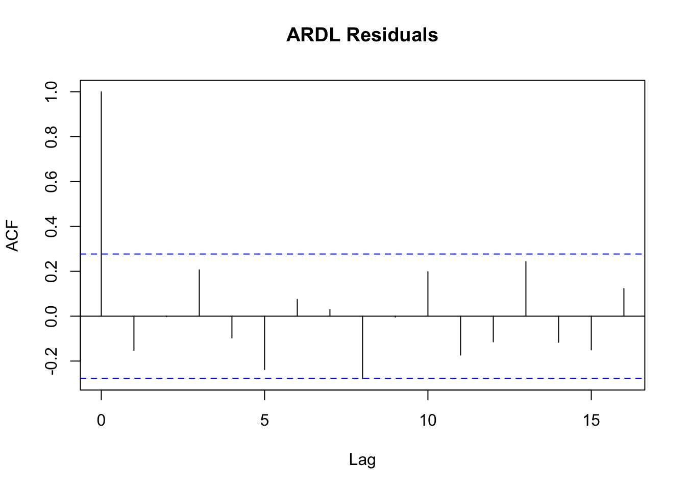
In the ACF plot, we see that the residuals do not have significant autocorrelation at any lag length. This gives evidence that the correct number of lags have been selected.
To check for Granger causality, we do a joint hypothesis test on the coefficients on both lags of a variable. To test whether \(SER2\) Granger causes \(DU\), we use the following hypotheses:
\[\begin{align*} H_0: & \gamma_{1} = 0, \gamma_{2} = 0\\ H_1: & \gamma_{1} \neq 0 \text{ and/or } \gamma_{2} \neq 0 \end{align*}\]
# Compute the SSR from the unrestricted (original model)
SSR_U = deviance(apap.ARDL)

# Compute the restricted model and retrieve its SSR
apap.GrangerSER <- dynlm(formula = du ~ L(du,1) + L(du,2) +
                   L(man2,1) + L(man2,2),
                   data = apap.ts)
SSR_SER = deviance(apap.GrangerSER)

# Compute the F statistic and its p-value
F_SER = (SSR_SER/SSR_U - 1) * (apap.ARDL$df.residual/2)
P_SER = df(F_SER,2,apap.ARDL$df.residual)
The F-statistic from this test is 0.1194 with corresponding p-value 0.8828. As the p-value is much greater than the \(5\%\) significance level, there is no evidence that \(SER2\) Granger causes \(DU\).
To test whether \(MAN2\) Granger causes \(DU\), we use the following hypotheses:
\[\begin{align*} H_0: & \delta_{1} = 0, \delta_{2} = 0\\ H_1: & \delta_{1} \neq 0 \text{ and/or } \delta_{2} \neq 0 \end{align*}\]
# Compute the SSR from the unrestricted (original model)
SSR_U = deviance(apap.ARDL)

# Compute the restricted model and retrieve its SSR
apap.GrangerMAN <- dynlm(formula = du ~ L(du,1) + L(du,2) +
                   L(ser2,1) + L(ser2,2),
                   data = apap.ts)
SSR_MAN = deviance(apap.GrangerMAN)

# Compute the F statistic and its p-value
F_MAN = (SSR_MAN/SSR_U - 1) * (apap.ARDL$df.residual/2)
P_MAN = df(F_MAN,2,apap.ARDL$df.residual)
The F-statistic from this test is 1.7753 with corresponding p-value 0.1678. As the p-value is much greater than the \(5\%\) significance level, there is no evidence that \(MAN2\) Granger causes \(DU\).
In the new Keynesian Phillips curve (NKPC), inflation at time \(t\) (\(INF_{t}\)) depends on inflationary expectations formed at time \(t\) for time \(t + 1\) (\(INFEX_{t}\)), and the output gap defined as output less potential output. Expectations of higher inflation lead to greater inflation. The closer output is to potential output, the higher the inflation rate. Amberger et al. compare results from estimating NKPCs with two output gaps, one that has been augmented with changes in financial variables (\(FNGAP_{t}\)), and one that has not (\(GAP_{t}\)). Quarterly data for Italy for the period 1990Q1 to 2014Q4 can be found in the data file
italy.
Using OLS, estimate the two equations
\[\begin{align} INF_{t} &= \alpha_{G} + \beta_{G}INFEX_{t} + \gamma_{G}GAP_{t} + e_{Gt}\\ INF_{t} &= \alpha_{F} + \beta_{F}INFEX_{t} + \gamma_{F}FNGAP_{t} + e_{Ft} \end{align}\]
Find \(95\%\) interval estimates for \(\gamma_{G}\) and \(\gamma_{F}\) using both conventional and HAC standard errors. Comment on (i) the relative widths of the intervals with and without HAC standard errors and (ii) whether one output gap measure is preferred over another in terms of its impact on inflation.
# Load the CSV in and convert to time series object
italy = read.csv("data/italy.csv")
italy.ts = ts(data = italy,
              start = 1,
              end = 100)


#################
### GAP MODEL ###
#################

# Estimate the model
reg.G= dynlm(data = italy.ts, formula = inf ~ infex + gap)

# Compute the HAC standard errors
hac.G = coeftest(reg.G, vcov = NeweyWest)

# Construct interval estimates of the two
crit = qt(0.975, reg.G$df.residual)
gammaG = reg.G$coefficients[3]

margin.olsG = crit * coeftest(reg.G)[6]
CI.olsG = c(gammaG - margin.olsG, gammaG + margin.olsG)

margin.hacG = crit * hac.G[6]
CI.hacG = c(gammaG - margin.hacG, gammaG + margin.hacG)

###################
### FNGAP MODEL ###
###################

# Estimate the model
reg.F= dynlm(data = italy.ts, formula = inf ~ infex + fngap)

# Compute the HAC standard errors
hac.F = coeftest(reg.F, vcov = NeweyWest)

# Construct interval estimates of the two
gammaF = reg.F$coefficients[3]

margin.olsF = crit * coeftest(reg.F)[6]
CI.olsF = c(gammaF - margin.olsF, gammaF + margin.olsF)

margin.hacF = crit * hac.F[6]
CI.hacF = c(gammaF - margin.hacF, gammaF + margin.hacF)
The regression output for the first model using conventional and HAC standard errors follow:
| term | estimate | std.error | statistic | p.value |
|---|---|---|---|---|
| (Intercept) | 0.0857 | 0.0912 | 0.9402 | 0.3494 |
| infex | 1.0157 | 0.0288 | 35.2594 | 0.0000 |
| gap | 0.1281 | 0.0349 | 3.6661 | 0.0004 |
| term | estimate | std.error | statistic | p.value |
|---|---|---|---|---|
| (Intercept) | 0.0857 | 0.2542 | 0.3372 | 0.7367 |
| infex | 1.0157 | 0.0745 | 13.6378 | 0.0000 |
| gap | 0.1281 | 0.0776 | 1.6517 | 0.1018 |
The regression output for the second model using conventional and HAC standard errors follow:
| term | estimate | std.error | statistic | p.value |
|---|---|---|---|---|
| (Intercept) | 0.1337 | 0.0916 | 1.459 | 0.1477 |
| infex | 0.9823 | 0.0304 | 32.266 | 0.0000 |
| fngap | 0.1256 | 0.0302 | 4.156 | 0.0001 |
| term | estimate | std.error | statistic | p.value |
|---|---|---|---|---|
| (Intercept) | 0.1337 | 0.2068 | 0.6462 | 0.5197 |
| infex | 0.9823 | 0.0715 | 13.7474 | 0.0000 |
| fngap | 0.1256 | 0.0712 | 1.7647 | 0.0808 |
The \(95\%\) confidence intervals for both models with both standard and HAC standard errors is given in the following table:
| Model G | Model F | |
|---|---|---|
| OLS | [0.0588, 0.1975] | [-0.0258, 0.282] |
| HAC | [0.0656, 0.1856] | [-0.0157, 0.2668] |
Both output gap variables have a similar impact on inflation. The interval estimates using HAC standard errors are slightly wider than those from conventional standard errors. This suggests that the precision of estimation will be overstated if we ignore the autocorrelation in the errors.
What are the values of the first four residual autocorrelations from each of the two regressions in part (a)? Which ones are significantly different from zero at a \(5\%\) significance level?
# Pull residuals from the G model and compute the autocorrelations
residG = resid(reg.G)
acG = acf(residG, pl=FALSE)

# Pull residuals from the F model and compute the autocorrelations
residF = resid(reg.F)
acF = acf(residF, pl=FALSE)

# Compute the 5% cutoff level
cR = 1.96/10
The first four residual autocorrelations for the models with GAP and FNGAP are given in the following table:
| r1 | r2 | r3 | r4 | |
|---|---|---|---|---|
| GAP | 0.6453 | 0.3776 | 0.2579 | 0.0322 |
| FNGAP | 0.6493 | 0.3795 | 0.2410 | -0.0043 |
The \(5\%\) critical value for a significant autocorrelation with 100 time periods is approximately \(\pm 0.196\).
As such, the first three residual autocorrelations in both models are significant at the \(5\%\) level.
Consider the generic equation \(y_{t} = \alpha + \beta x_{t} + \gamma z_{t} + e_{t}\) with AR(2) errors \(e_{t} = \Psi_{1}e_{t - 1} + \Psi_{2}e_{t - 2} + v_{t}\) where the \(v_{t}\) are not autocorrelated. Show that this model can be written as
\[ y_{t}^{*} = \alpha^{*} + \beta x_{t}^{*} + \gamma z_{t}^{*} + v_{t} \qquad t = 3, 4, \dots, T \]
where
\[\begin{align*} y_{t}^{*} &= y_{t} - \Psi_{1}y_{t - 1} - \Psi_{2}y_{t - 2}\\ \alpha^{*} &= \alpha(1 - \Psi_{1} - \Psi_{2})\\ x_{t}^{*} &= x_{t} - \Psi_{1}x_{t - 1} - \Psi_{2}x_{t - 2}\\ z_{t}^{*} &= z_{t} - \Psi_{1}z_{t - 1} - \Psi_{2}z_{t - 2} \end{align*}\]
The process for this follows a similar process as 9.32(c). We first rewrite the error in the original equation in its AR(2) form:
\[ y_{t} = \alpha + \beta x_{t} + \gamma z_{t} + \Psi_{1}e_{t - 1} + \Psi_{2}e_{t - 2} + v_{t} \]
Next, iterate the model back to \(t - 1\) and \(t - 2\) and solve for the error in each period:
\[\begin{align*} y_{t-1} &= \alpha + \beta x_{t-1} + \gamma z_{t -1} + e_{t - 1} \longrightarrow e_{t - 1} = y_{t-1} - \left(\alpha + \beta x_{t-1} + \gamma z_{t-1}\right)\\ y_{t-2} &= \alpha + \beta x_{t-2} + \gamma z_{t -2} + e_{t - 2} \longrightarrow e_{t - 2} = y_{t-2} - \left(\alpha + \beta x_{t-2} + \gamma z_{t-2}\right)\\ \end{align*}\]
Next plug both error formulas into the equation for period \(t\) with AR(2) error:
\[\begin{align*} y_{t} = &\alpha + \beta x_{t} + \gamma z_{t} + v_{t}\\ &+\Psi_{1}\left[y_{t-1} - \left(\alpha + \beta x_{t-1} + \gamma z_{t-1}\right)\right]\\ &+\Psi_{2}\left[y_{t-2} - \left(\alpha + \beta x_{t-2} + \gamma z_{t-2}\right)\right]\\ \end{align*}\]
Moving the \(y_{t - 1}\) and \(y_{t - 2}\) terms to the LHS and grouping the constant, \(x\), and \(z\) terms together will yield the desired result.
Using the least squares residuals \(\hat{e}_{Gt}\) from the first equation in part (a), estimate \(\Psi_{1}\) and \(\Psi_{2}\) from the regression equation \(\hat{e}_{Gt} = \Psi_{1}\hat{e}_{Gt-1} + \Psi_{2}\hat{e}_{Gt - 2} + \hat{v}_{t}\). Along the lines of the transformations in part (c), use the estimates of \(\Psi_{1}\) and \(\Psi_{2}\) to find transformed variables \(INF_{t}^{*}\), \(INFEX_{t}^{*}\), and \(GAP_{t}^{*}\), and then estimate \(\alpha_{G}^{*}\), \(\beta_{G}\), and \(\gamma_{G}\) from the transformed equation \(INF_{t}^{*} = \alpha_{G}^{*} + \beta_{G}INFEX_{t}^{*} + \gamma_{G}GAP_{t}^{*} + v_{t}\). Estimate the equation with both conventional and HAC standard errors.
# Estimate the AR(2) error process
reg.ar = dynlm(residG ~ 0 + L(residG,1) + L(residG,2))
psi1 = reg.ar$coefficients[1]
psi2 = reg.ar$coefficients[2]

# Apply transformations and create a new time series object
inf   <- italy.ts[3:100,"inf"] - psi1*italy.ts[2:99,"inf"]-
         psi2*italy.ts[1:98,"inf"]
infex <- italy.ts[3:100,"infex"] - psi1*italy.ts[2:99,"infex"]-
         psi2*italy.ts[1:98,"infex"]
gap   <- italy.ts[3:100,"gap"] - psi1*italy.ts[2:99,"gap"]-
         psi2*italy.ts[1:98,"gap"]

trans.ts <- ts(cbind(inf,infex,gap))

# Estimate the model
reg.trans= dynlm(data = trans.ts, formula = inf ~ infex + gap)

# Compute the HAC standard errors
hac.trans = coeftest(reg.trans, vcov = NeweyWest)
The regression output for the model with transformed variables using conventional and HAC standard errors follow:
| term | estimate | std.error | statistic | p.value |
|---|---|---|---|---|
| (Intercept) | 0.0743 | 0.0633 | 1.173 | 0.2439 |
| infex | 0.9670 | 0.0581 | 16.638 | 0.0000 |
| gap | 0.0577 | 0.0489 | 1.180 | 0.2409 |
| term | estimate | std.error | statistic | p.value |
|---|---|---|---|---|
| (Intercept) | 0.0743 | 0.0766 | 0.9698 | 0.3346 |
| infex | 0.9670 | 0.0807 | 11.9835 | 0.0000 |
| gap | 0.0577 | 0.0520 | 1.1097 | 0.2699 |
Using the results from part (d), find \(95\%\) interval estimates for \(\gamma_{G}\) using both conventional and HAC standard errors. Comment on (i) the relative widths of the intervals with and without HAC standard errors, and (ii) how the estimates and intervals compare with the corresponding ones obtained in part (a).
# Construct interval estimates with both standard errors
crit = qt(0.975, reg.trans$df.residual)
gammaG = reg.trans$coefficients[3]

margin.olsTrans = crit * coeftest(reg.trans)[6]
CI.olsTrans = c(gammaG - margin.olsTrans, gammaG + margin.olsTrans)

margin.hacTrans = crit * hac.trans[6]
CI.hacTrans = c(gammaG - margin.hacTrans, gammaG + margin.hacTrans)
The confidence interval for \(\gamma_{G}\) computed using OLS standard errors is \([-0.0393, 0.1547]\). The confidence interval for \(\gamma_{G}\) computed using the HAC standard errors is \([-0.0455, 0.1608]\). The width from the HAC standard errors is slightly wider than that from the conventional standard. However, this difference is not as large as the difference in widths from the results in part (a). The most dramatic change comes from the point estimate of \(\gamma_{G}\) itself. After the transformation of variables, the estimate for \(\gamma_{G}\) has dropped from \(0.1291\) to \(0.0577\). As discussed earlier, the GLS method requires a stronger exogeneity assumption than the estimates in part (a), so this large change could come from a violation of this assumption.
Thank you to Coleman Cornell for generously sharing his materials with me.