Midterm 1 Questions and Answers
Worked Solutions with Explanations
A Note on Versions
There are two versions. This follows the “blue” version, and I will put the purple version question numbers and the answers in parentheses. CAE exams are blue exams (though they were printed on white paper)
Question 1
(Purple Version Question 8)
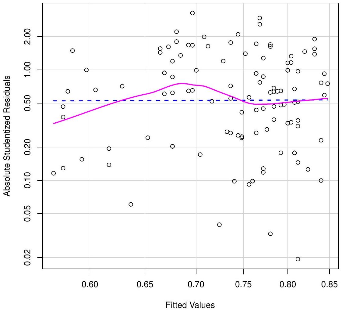
Which statement about the Spread Level plot below is correct?
- The plot shows a clear upward trend in the spread of residuals as the fitted values increase, indicating the presence of heteroskedasticity.
- The plot displays a systematic pattern in the spread of residuals, suggesting that the variance of the error term depends on the level of the explanatory variable.
- The plot shows a nonlinear relationship between the residuals and the fitted values, implying that the model suffers from heteroskedasticity.
- The plot indicates that the spread of residuals is approximately constant across fitted values, providing no evidence of heteroskedasticity.
Correct Answers (Blue / Purple): (d) / (b)
In the spread-level plot:
- The points are fairly evenly scattered with no funnel shape.
- The smooth (pink) line is nearly flat and stays close to the horizontal reference line.
- There’s no consistent increase or decrease in spread as fitted values change.
All of this suggests constant variance of the residuals, so there’s no evidence of heteroskedasticity.
Question 2
(Purple Version Question 9)
The R code below tests for heteroskedasticity in a wage equation: \[\text{wage} = \beta_0 + \beta_1 \text{educ} + \beta_2 \text{exper} + e\]
Based on the output, what can you conclude at the 5% significance level?
> model <- lm(wage ~ educ + exper, data = wage_data)
> bptest(model)
    studentized Breusch-Pagan test
data: model
BP = 14.236, df = 2, p-value = 0.0008103- Fail to reject \(H_0\); no evidence of heteroskedasticity
- Reject \(H_0\); heteroskedasticity is present
- The test is inconclusive
- The p-value is too large to make a conclusion
Correct Answers (Blue / Purple): (b) / (c)
The Breusch-Pagan test:
- \(H_0\): Homoskedasticity (no heteroskedasticity)
- \(H_a\): Heteroskedasticity is present
- Test statistic: \(BP = 14.236\)
- p-value \(= 0.0008103 < 0.05\)
Since p-value \(< 0.05\), we reject \(H_0\) and conclude heteroskedasticity is present.
Key Point: BP test uses \(n \times R^2\) from regressing \(\hat{e}_i^2\) on regressors.
Question 3
(Purple Version Question 10)
For the food expenditure data, the estimated model with robust (White) standard errors is:
\[ \begin{aligned} \widehat{\text{food\_exp}} = & 83.42 + 10.21 \cdot \text{income} \\ & (27.46) \quad (1.81) \quad \text{White se} \\ & (43.41) \quad (2.09) \quad \text{Incorrect se} \end{aligned} \]
Calculate the 95% confidence interval for \(\beta_2\) using White standard errors. Assume \(t_c = 2.024\).
- \([5.97, 14.45]\)
- \([9.36, 11.06]\)
- \([7.89, 12.53]\)
- \([6.55, 13.87]\)
Correct Answers (Blue / Purple): (d) / (a)
Calculation using White standard errors:
\[ \begin{aligned} CI & = b_2 \pm t_c \times se(b_2) \\ & = 10.21 \pm 2.024 \times 1.81 \\ & = 10.21 \pm 3.66 \\ & = [6.55, 13.87] \end{aligned} \]
Common Error: Using incorrect (OLS) standard errors: \[10.21 \pm 2.024 \times 2.09 = [5.97, 14.45]\] which is option (a) (b).
Question 4
(Purple Version Question 11)
Consider the Coke demand model: \[\text{coke} = \beta_1 + \beta_2 \cdot \text{pratio} + \beta_3 \cdot \text{disp\_coke} + \beta_4 \cdot \text{disp\_pepsi} + e\]
The R code below estimates this model:
coke.ols <- lm(coke ~ pratio + disp_coke + disp_pepsi, data=coke)
coke.hc1 <- coeftest(coke.ols, vcov.=hccm(coke.ols, type="hc1"))
What does type=“hc1” specify?
- First-order autocorrelation correction
- Homoskedasticity test statistic
- Heteroskedasticity-consistent (White) standard errors with finite sample adjustment
- Weighted Least Squares transformation
Correct Answers (Blue / Purple): (c) / (d)
In R’s hccm() function:
hc0: White’s original heteroskedasticity-consistent estimatorhc1: HC0 with finite sample correction: multiply by \(N/(N-K)\)hc2,hc3: Other variants
HC1 is commonly used because it performs better in finite samples.
Question 5
(Purple Version Question 12)
The R code below estimates a weighted least squares (WLS) regression. In R, the weights argument determines how observations are weighted in the objective function. Based on this implementation, what weight is effectively applied to each observation?
w <- 1/food$income
reg.mod.wls <- lm(food_exp ~ income, weights=w, data=food)- \(w_i = \text{income}_i\)
- \(w_i = \sqrt{\text{income}_i}\)
- \(w_i = 1/\text{income}_i\)
- \(w_i = 1/\sqrt{\text{income}_i}\)
Correct Answers (Blue / Purple): (d) / (b)
In R’s lm() function with weights:
- R automatically takes the square root of the weights
- If you specify
weights=w, R uses \(\sqrt{w}\) as the divisor - So \(w = 1/\text{income}\) means R divides by \(\sqrt{1/\text{income}} = 1/\sqrt{\text{income}}\)
Key Point: R’s weights argument specifies \(w_i\) where \(\text{Var}(\epsilon_i) = \sigma^2/w_i\). The effective transformation divides by \(\sqrt{w_i}\).
The answer key mistakenly had 1/\(\text{income}_i\) as the answer, but then was corrected to 1/\(\sqrt{\text{income}_i}\).
Question 6
(Purple Version Question 13)
Below is output from testing heteroskedasticity using a residual regression. The original model is \(\text{price} = \beta_0 + \beta_1 \text{sqft} + \beta_2 \text{bdrms} + e\). Using the Breusch-Pagan LM test, what is the value of the test statistic? Assume \(n=88\).
Residual standard error: 1845 on 85 degrees of freedom
Multiple R-squared: 0.0847, Adjusted R-squared: 0.0632- \(\chi^2 = 7.45\)
- \(\chi^2 = 0.0847\)
- \(\chi^2 = 3.932\)
- \(\chi^2 = 0.02329\)
Correct Answers (Blue / Purple): (a)
For the Breusch-Pagan test: \[\chi^2 = n \times R^2 = 88 \times 0.0847 = 7.4536\]
This is compared to \(\chi^2_{df=2}\) critical value.
Key Points:
- BP test statistic \(= N \times R^2\) from auxiliary regression
- \(R^2 = 0.0847\) (not the F-statistic or p-value)
- df = number of regressors in auxiliary regression (excluding intercept) = 2
Question 7
(Purple Version Question 14)
Consider estimating the variance function: \(\sigma_i^2 = \sigma^2 x_i^\gamma\) where \(\gamma\) is unknown. To estimate \(\gamma\), we take logs and get: \[\ln(\sigma_i^2) = \ln(\sigma^2) + \gamma \ln(x_i) = \alpha_1 + \alpha_2 \ln(x_i)\]
In the FGLS procedure, what do we regress on \(\ln(x_i)\) to estimate \(\gamma\)?
- \(\hat{e}_i^2\)
- \(|\hat{e}_i|\)
- \(\ln(\hat{e}_i^2)\)
- \(\hat{e}_i\)
Correct Answers (Blue / Purple): (c) / (d)
FGLS procedure for unknown variance form:
- Estimate original model by OLS, get residuals \(\hat{e}_i\)
- To estimate variance function \(\ln(\sigma_i^2) = \alpha_1 + \alpha_2 \ln(x_i)\)
- Regress \(\ln(\hat{e}_i^2)\) on \(\ln(x_i)\): \(\ln(\hat{e}_i^2) = \alpha_1 + \alpha_2 \ln(x_i) + v_i\)
- Get \(\hat{\sigma}_i^2 = \exp(\hat{\alpha}_1 + \hat{\alpha}_2 \ln(x_i))\)
- Apply WLS using \(w_i = 1/\hat{\sigma}_i\)
Key Point: We take logs of both sides, so we need \(\ln(\hat{e}_i^2)\) on the LHS.
Question 8
(Purple Exam Question 6)
After fitting a linear regression model, you examine a residuals-versus-fitted-values plot and observe a clear reverse funnel shape: the residuals have large spread at small fitted values and progressively smaller spread at larger fitted values. Which test is most appropriate for formally assessing heteroskedasticity in this situation?
- The Breusch-Pagan test, because it tests whether the error variance depends on specific regressors in the model.
- The non-constant variance score test (
ncvTest()), because it tests whether the error variance is a function of the fitted values, regardless of whether the variance increases or decreases.
- The White test, because it detects serial correlation in the regression residuals.
- The Jarque-Bera test, because it assesses whether the residuals are normally distributed.
Correct Answers (Blue / Purple): (b) / (c)
That is exactly the setting where ncvTest() is more appropriate than bptest().
Key Differences:
- BP test: Tests if variance depends on specific regressors \(x_j\)
- NCV test: Tests if variance depends on fitted values \(\hat{y}\) (any continuous function)
- White test: General test using squares and cross-products of regressors
- Jarque-Bera: Tests normality (not heteroskedasticity)
The reverse funnel shape (variance changing with fitted values) is what NCV test is designed to detect.
Question 9
(Purple Exam Question 7)
Below we estimate a consumption function with robust (White) standard errors. Which coefficient’s confidence interval has relatively widened the most compared to OLS?
Coefficients (OLS standard errors):
            Estimate Std. Error
(Intercept)  124.58    45.23
income         0.85     0.12
wealth         0.043    0.015

Coefficients (White standard errors):
            Estimate Std. Error
(Intercept)  124.58    52.10
income         0.85     0.18
wealth 0.043 0.012- Intercept
- income
- wealth
- They all widened equally
Correct Answers (Blue / Purple): (b) / (c)
Compare standard error changes:
- Intercept: \(52.10 / 45.23 = 1.152\) (15.2% increase)
- income: \(0.18 / 0.12 = 1.500\) (50% increase) \(\leftarrow\) Largest
- wealth: \(0.012 / 0.015 = 0.800\) (20% decrease)
The income coefficient’s confidence interval widened most (50% increase in standard error).
Key Point: Robust SEs can be larger or smaller than OLS SEs. Here, wealth actually got more precise with robust SEs.
Question 10
(Purple Exam Question 2)
Which statement about the ncvTest is correct?
- The
ncvTesttests \(\sigma_i^2 = \sigma^2 x_i\)
- The
ncvTesttests \(\sigma_i^2 = \sigma^2 x_i^\gamma\)
- The
ncvTesttests \(\sigma_i^2 = \sigma^2 f(\widehat{y})\), where \(f()\) is a continuous function
- The
ncvTesttests \(\sigma_i^2 = \sigma^2 h(\alpha_0 + \alpha_1 x_1 + \cdots + \alpha_s x_s)\)
Correct Answers (Blue / Purple): (c) / (d)
Recall that this test is based on \(\sigma_i^2 = \sigma^2 f(\widehat{y})\), where \(f()\) is a continuous function.
As such, it does not suffer from the same issues as e.g., the BP Test which requires specifying particular regressors.
Key Advantage: NCV test is more flexible — it detects heteroskedasticity related to fitted values without assuming a specific functional form.
Question 11
(Purple Exam Question 3)
For the model \(y = \beta_0 + \beta_1 x + e\) with \(\text{Var}(e_i) = \sigma^2 x_i^2\), the appropriate weight for WLS estimation is:
- \(w_i = 1/x_i\)
- \(w_i = x_i\)
- \(w_i = x_i^2\)
- \(w_i = 1/x_i^2\)
Correct Answers (Blue / Purple): (a) / (a)
With \(\text{Var}(e_i) = \sigma^2 x_i^2\), we have \(\sigma_i = \sigma x_i\).
For WLS, we transform by dividing by the standard deviation: \[w_i = \frac{1}{\sigma_i} = \frac{1}{\sigma x_i}\]
The effective transformation weight is \(1/x_i\).
Note: This is a subtle question. If we specify weights in R as \(1/x_i^2\), R takes the square root and divides by \(1/x_i\).
Question 12
(Purple Exam Question 1)
The White test differs from the Breusch-Pagan test in that it:
- Is more powerful for detecting heteroskedasticity
- Requires a larger sample size
- Tests for serial correlation instead of heteroskedasticity
- Includes squared and cross-product terms of the regressors
Correct Answers (Blue / Purple): (d) / (a)
White test vs. Breusch-Pagan:
- BP test: Regresses \(\hat{e}_i^2\) on original regressors \(x_2, \ldots, x_K\)
- White test: Regresses \(\hat{e}_i^2\) on \(x_2, \ldots, x_K\), their squares \(x_2^2, \ldots, x_K^2\), and cross-products \(x_2 x_3, \ldots\)
- White test is more general (doesn’t assume specific form)
Key Point: White test includes squared and cross-product terms to capture more general forms of heteroskedasticity.
Question 13
(Purple Exam Question 4)
Below we model heteroskedasticity as \(\sigma_i^2 = \sigma^2 e^{\alpha_0 + \alpha_1 x_i}\). The R output shows the estimation of the variance function. What is the estimated value of \(\alpha_1\)?
> var_model <- lm(log(resid_sq) ~ x)
> summary(var_model)
Coefficients:
            Estimate Std. Error t value Pr(>|t|)
(Intercept)  2.3456     0.4521   5.187  1.2e-06 ***
x            0.0852     0.0234   3.641  0.00042 ***
---
Residual standard error: 1.234 on 98 degrees of freedom
Multiple R-squared: 0.1192, Adjusted R-squared: 0.1102- 2.3456
- 1.234
- 0.1192
- 0.0852
Correct Answers (Blue / Purple): (d) / (d)
The model is: \[\log(\sigma_i^2) = \alpha_0 + \alpha_1 x_i\]
or equivalently \(\sigma_i^2 = e^{\alpha_0 + \alpha_1 x_i}\).
From the output, the coefficient on \(x\) is \(\hat{\alpha}_1 = 0.0852\).
Key Point: In the log-variance regression, the slope coefficient gives us \(\alpha_1\) directly.
Question 14
(Purple Exam Question 5)
An analyst is comparing models for stock prices and stock returns. The analyst wants a model in which the estimated coefficients have a stable interpretation and do not depend on the particular time window used in the sample, so that standard inference is meaningful. Which property of a time series best supports this goal?
- The series has parameters that change as the sample grows, reflecting the accumulation of shocks over time.
- The series has coefficients that depend strongly on the chosen sample window rather than remaining stable across subsamples.
- The series exhibits long-run trending behavior, making recent observations more informative than older ones.
- The series is covariance stationary, so its mean, variance, and autocovariances are constant over time.
Correct Answers (Blue / Purple): (d) / (d)
Covariance stationarity ensures that the mean, variance, and dependence structure of the series are stable over time, so estimated coefficients do not change with the sample window and standard statistical inference is valid.
Why others are wrong:
- Changing parameters make inference invalid
- Unstable coefficients mean unreliable estimates
- Trending behavior violates stationarity
Key Point: Stationarity is required for valid time series inference.
Question 15
(Purple Exam Question 22)
The Goldfeld-Quandt (GQ) test for heteroskedasticity was performed on the food expenditure model with the following R code:
> gqtest(reg.mod, point=0.5, alternative="greater",
+        order.by=food$income)
    Goldfeld-Quandt test
data: reg.mod
GQ = 3.8214, df1 = 18, df2 = 18, p-value = 0.002609
What does this test do?
- Tests for normality of residuals
- Compares variances of two subsamples split by median income
- Tests for serial correlation
- Compares means of two subsamples
Correct Answers (Blue / Purple): (b) / (c)
Goldfeld-Quandt test procedure:
- Order observations by the variable suspected of causing heteroskedasticity (
order.by=food$income) - Split sample at a point (
point=0.5means median) - Omit middle observations
- Estimate separate regressions for low and high groups
- Calculate \(F = SSE_{\text{high}} / SSE_{\text{low}}\) (ratio of variances)
- If \(F\) is large (
alternative="greater"), reject homoskedasticity
With p-value \(= 0.002609 < 0.05\), we reject \(H_0\) and conclude heteroskedasticity is present.
Question 16
(Purple Exam Question 23)
Below we estimate an AR(2) model for inflation (\(INF_t\)). What is the one-step-ahead forecast for period \(T+1\) if \(INF_T = 2.5\) and \(INF_{T-1} = 3.0\)?
Call:
dynlm(formula = inf_ts ~ L(inf_ts, 1:2))
Coefficients:
            Estimate Std. Error t value Pr(>|t|)
(Intercept)  0.4523     0.1876   2.411   0.0178 *
L(inf_ts,1)  0.6234     0.0945   6.595 2.1e-09 ***
L(inf_ts,2)  0.2145     0.0982   2.184   0.0312 *
---
Residual standard error: 0.8234 on 87 df- 2.6543
- 3.1526
- 2.0000
- 1.7526
Correct Answers (Blue / Purple): (a) / (b)
The AR(2) model is: \[INF_t = 0.4523 + 0.6234 \times INF_{t-1} + 0.2145 \times INF_{t-2}\]
One-step-ahead forecast for \(T+1\): \[\begin{aligned} \widehat{INF}_{T+1} &= 0.4523 + 0.6234(2.5) + 0.2145(3.0) \\ &= 0.4523 + 1.5585 + 0.6435 \\ &= 2.6543 \end{aligned}\]
Key Point: Use the estimated coefficients and the two most recent observed values.
Question 17
(Purple Exam Question 24)
The first-order sample autocorrelation \(r_1\) for GDP growth \(G_t\) is calculated as: \[r_1 = \frac{\sum_{t=2}^{T}(G_t - \bar{G})(G_{t-1} - \bar{G})}{\sum_{t=2}^{T}(G_t - \bar{G})^2}\]
This measures the correlation between:
- \(G_t\) and \(G_{t-1}\) (observations one period apart)
- \(G_t\) and time \(t\)
- \(G_t\) and \(\Delta G_t\)
- \(G_t\) and the residuals
Correct Answers (Blue / Purple): (a) / (b)
First-order autocorrelation:
- Measures correlation between a variable and its first lag
- \(r_1 =\) correlation between \(G_t\) and \(G_{t-1}\)
- “First-order” means lag 1 (one period apart)
- General: \(r_k =\) correlation between \(G_t\) and \(G_{t-k}\)
From Chapter 9: “\(\rho_1\) is used to denote the population correlation between observations that are one period apart in time. This is known also as the population autocorrelation of order one.”
Question 18
(Purple Exam Question 25)
For the Phillips Curve model using phillips5_aus data, we regress inflation (inf) on change in unemployment (Du):
inf.ts <- phillips5_aus.ts[,"inf"]
Du.ts <- diff(phillips5_aus.ts[,"u"])
reg.ts = dynlm(inf.ts ~ Du.ts, data=phillips5_aus.ts)
An ACF plot of the residuals shows significant spikes at lags 1 and 2. This suggests:
- The model is correctly specified
- The data are non-stationary
- Serial correlation is present; the model may be missing dynamics
- Heteroskedasticity is present
Correct Answers (Blue / Purple): (c) / (d)
ACF plot interpretation:
- If model is correctly specified: Residuals should be white noise
- White noise: ACF should show no significant spikes (except at lag 0)
- Significant spikes at lags 1-2: Residuals are autocorrelated
- This suggests: Model hasn’t captured all the dynamics
- Solution: Add lagged variables (e.g., use ARDL instead)
Key Point: Significant ACF spikes in residuals indicate serial correlation and model misspecification.
The answer key mistakenly had “Heteroskedasticity” as the correct answer, but it is actually “Serial Correlation is present; the model may be missing dynamics”.
Question 19
(Purple Exam Question 20)
For an AR(2) model, the 95% interval forecast for \(j\) periods ahead is: \[\widehat{G}_{T+j} \pm t_{(0.975, df)} \cdot \widehat{\sigma}_j\]
As \(j\) increases (forecasting further into the future), what happens to \(\widehat{\sigma}_j\)?
- It decreases (narrower intervals)
- It increases (wider intervals)
- It remains constant
- It depends on the sign of the AR coefficients
Correct Answers (Blue / Purple): (b) / (c)
For AR models, forecast uncertainty grows as we forecast further ahead:
- \(\widehat{\sigma}_j\) increases with \(j\)
- Intuition: Each forecast depends on previous forecasts, accumulating uncertainty
- Mathematically: \(\widehat{\sigma}_j^2 = \sigma^2(1 + \psi_1^2 + \psi_2^2 + \cdots + \psi_{j-1}^2)\) where \(\psi\) are MA coefficients
- Result: Forecast intervals get wider as forecast horizon increases
Key Point: Forecast uncertainty compounds over time in AR models.
Question 20
(Purple Exam Question 21)
Below we compare AR models using information criteria. Which model should be selected based on BIC?
| Model | AIC | BIC |
|---|---|---|
| AR(1) | 245.23 | 252.45 |
| AR(2) | 242.18 | 252.67 |
| AR(3) | 241.95 | 255.71 |
| AR(4) | 240.23 | 257.26 |
- AR(1)
- AR(2)
- AR(3)
- AR(4)
Correct Answers (Blue / Purple): (a) / (b)
Choose model with lowest BIC:
- AR(1): BIC = 252.45 ← Lowest
- AR(2): BIC = 252.67
- AR(3): BIC = 255.71
- AR(4): BIC = 257.26
BIC penalizes model complexity more heavily than AIC, favoring simpler models.
Key Point: For model selection, choose the model with the lowest information criterion value.
Question 21
(Purple Exam Question 16)
Consider an AR(2) model for GDP growth: \[G_t = \delta + \theta_1 G_{t-1} + \theta_2 G_{t-2} + v_t\]
Estimated results give: \(\hat{\delta}=0.67, \hat{\theta}_1=0.12, \hat{\theta}_2=-0.09\). If \(G_T=0.8\) and \(G_{T-1}=-0.2\), what is the one-step-ahead forecast \(\hat{G}_{T+1}\)?
- 0.84
- 0.69
- 0.78
- 0.75
Correct Answers (Blue / Purple): (c) / (d)
AR(2) forecast calculation: \[\hat{G}_{T+1} = \hat{\delta} + \hat{\theta}_1 G_T + \hat{\theta}_2 G_{T-1}\]
\[\hat{G}_{T+1} = 0.67 + 0.12(0.8) + (-0.09)(-0.2) = 0.67 + 0.096 + 0.018 = 0.784 \approx 0.78\]
Key Point: Use the most recent observed values and estimated coefficients.
Question 22
(Purple Exam Question 15)
The R code below estimates a model using dynlm:
model = dynlm(d(u_ts) ~ L(g_ts, 0:5))What model is being estimated?
- AR(5) model for \(u\)
- Regression of \(\Delta U_t\) on \(G_t, G_{t-1}, \ldots, G_{t-5}\)
- ARDL(5,5) model
- Regression of \(U_t\) on lagged \(G_t\)
Correct Answers (Blue / Purple): (b) / (c)
The R code dynlm(d(u_ts) ~ L(g_ts, 0:5)) means:
d(u_ts): First difference of \(u_t\) series = \(\Delta U_t\)L(g_ts, 0:5): \(G_t\) (lag 0) through \(G_{t-5}\) (lag 5)- Model: \(\Delta U_t = \beta_0 + \beta_1 G_t + \beta_2 G_{t-1} + \cdots + \beta_6 G_{t-5} + e_t\)
Key Point: L(x, 0:5) includes current value and 5 lags.
Question 23
(Purple Exam Question 17)
The R code below estimates an ARDL model. Which specification is being estimated?
model <- dynlm(du_ts ~ L(du_ts, 1) + L(g_ts, 0:1))- ARDL(1,0)
- ARDL(0,1)
- ARDL(1,1)
- ARDL(2,1)
Correct Answers (Blue / Purple): (c) / (a)
The R code dynlm(du_ts ~ L(du_ts, 1) + L(g_ts, 0:1)) means:
du_ts: Dependent variable is \(DU_t\)L(du_ts, 1): One lag of \(DU_t\) = \(DU_{t-1}\)L(g_ts, 0:1): \(G_t\) (lag 0) and \(G_{t-1}\) (lag 1)- Model: \(DU_t = \beta_0 + \beta_1 DU_{t-1} + \beta_2 G_t + \beta_3 G_{t-1} + e_t\)
This is ARDL(1,1): 1 lag of dependent variable, 1 lag of independent variable (plus current).
Key Point: ARDL(p,q) has p lags of dependent variable, q lags of independent variable.
Question 24
(Purple Exam Question 18)
Based on question 23, below we test for serial correlation in an ARDL model’s residuals using the Breusch-Godfrey test of order up to 4 (bgtest(ardl_model, order = 4)). Which auxiliary regression is used for the BG test?
Let \(\hat{e}_t\) be the OLS residual from the estimated ARDL model. \(du_t\) is the change in unemployment and \(g_t\) is GDP growth.
- \(\hat{e}_t = \gamma_0 + \gamma_1 du_{t-1} + \gamma_2 g_t + \gamma_3 g_{t-1} + \rho \hat{e}_{t-1} + v_t\)
- \(\hat{e}_t = \gamma_0 + \rho_1 \hat{e}_{t-1} + \rho_2 \hat{e}_{t-2} + \rho_3 \hat{e}_{t-3} + \rho_4 \hat{e}_{t-4} + v_t\)
- \(\hat{e}_t = \gamma_0 + \gamma_1 du_{t-1} + \gamma_2 g_t + \gamma_3 g_{t-1} + \rho_1 \hat{e}_{t-1} + \rho_2 \hat{e}_{t-2} + \rho_3 \hat{e}_{t-3} + \rho_4 \hat{e}_{t-4} + v_t\)
- \(\Delta \hat{e}_t = \gamma_0 + \gamma_1 \Delta du_{t-1} + \gamma_2 \Delta g_t + \gamma_3 \Delta g_{t-1} + \rho_1 \Delta \hat{e}_{t-1} + \rho_2 \Delta \hat{e}_{t-2} + \rho_3 \Delta \hat{e}_{t-3} + \rho_4 \Delta \hat{e}_{t-4} + v_t\)
Correct Answers (Blue / Purple): (c) / (c)
Breusch-Godfrey test procedure:
- Estimate original model, get residuals \(\hat{e}_t\)
- Run auxiliary regression: \(\hat{e}_t\) on all regressors from original model + lagged residuals
- For ARDL with \(du_{t-1}, g_t, g_{t-1}\): include these + \(\hat{e}_{t-1}, \hat{e}_{t-2}, \hat{e}_{t-3}, \hat{e}_{t-4}\)
- Test: \(H_0: \rho_1 = \rho_2 = \rho_3 = \rho_4 = 0\) (no serial correlation)
- Use \(LM = n \times R^2\) from auxiliary regression
Key Point: BG test includes original regressors + lagged residuals in auxiliary regression.
Question 25
(Purple Exam Question 19)
For an ARDL(1,1) model of inflation: \[INF_t = \delta + \theta_1 INF_{t-1} + \delta_0 DU_t + \delta_1 DU_{t-1} + v_t\]
The estimated results are:
| Estimate | |
|---|---|
| (Intercept) | 0.3336 |
| INF_t-1 | 0.5593 |
| DU_t | -0.6882 |
| DU_t-1 | 0.3200 |
What is the impact multiplier (immediate effect of \(DU_t\) on \(INF_t\))?
- -0.6882
- 0.5593
- -0.3682
- 0.3336
Correct Answers (Blue / Purple): (a) / (b)
In ARDL(1,1), three types of multipliers:
- Impact multiplier: \(\delta_0 =\) immediate effect of \(DU_t\) on \(INF_t\)
- Interim multiplier: \(\delta_0 + \delta_1 =\) effect after 1 period
- Long-run multiplier: \(\frac{\delta_0 + \delta_1}{1 - \theta_1} =\) cumulative effect
From estimates: Impact multiplier \(= \hat{\delta}_0 = -0.6882\)
Interpretation: A 1-unit increase in \(DU_t\) immediately reduces \(INF_t\) by 0.6882.
Answer Key Table
| Blue (V1) Q# | Blue Answer | Purple (V2) Q# | Purple Answer |
|---|---|---|---|
| 1 | D | 1 | A |
| 2 | B | 2 | D |
| 3 | D | 3 | A |
| 4 | C | 4 | C |
| 5 | D | 5 | D |
| 6 | A | 6 | C |
| 7 | C | 7 | C |
| 8 | B | 8 | B |
| 9 | B | 9 | C |
| 10 | C | 10 | A |
| 11 | A | 11 | D |
| 12 | D | 12 | B |
| 13 | C | 13 | B |
| 14 | D | 14 | D |
| 15 | B | 15 | C |
| 16 | A | 16 | D |
| 17 | A | 17 | A |
| 18 | C | 18 | D |
| 19 | B | 19 | B |
| 20 | A | 20 | C |
| 21 | C | 21 | B |
| 22 | B | 22 | C |
| 23 | C | 23 | B |
| 24 | C | 24 | B |
| 25 | A | 25 | D |