Call:
lm(formula = test_score ~ prior_grade, data = data)

Residuals:
    Min      1Q  Median      3Q     Max
-31.380  -4.997   0.532   6.055  28.079

Coefficients:
            Estimate Std. Error t value Pr(>|t|)
(Intercept) 40.72153    1.37453   29.63   <2e-16 ***
prior_grade  0.64043    0.01936   33.08   <2e-16 ***
---
Signif. codes:  0 '***' 0.001 '**' 0.01 '*' 0.05 '.' 0.1 ' ' 1

Residual standard error: 8.987 on 998 degrees of freedom
Multiple R-squared:  0.5231,    Adjusted R-squared:  0.5226
F-statistic: 1095 on 1 and 998 DF, p-value: < 2.2e-164 Omitted Variable Bias
What Happens When You Leave Out a Relevant Variable
Endogeneity
OLS Assumptions
Cross-Section
NotePrerequisites
This chapter assumes familiarity with OLS estimation and heteroskedasticity. For the solution to endogeneity, see Instrumental Variables.
The assumptions of Simple1 Linear Regression under random sampling are the following:
| Assumption | Description |
|---|---|
| RS1 | The model is linear, i.e. \(y_{i}=\beta_{1}+\beta_{2} x_{i}+e_{i}\) |
| RS2 | The data pairs \(\left(y_{i}, x_{i}\right)\) are independent and identically distributed (iid). |
| RS3 | Exogeneity: \(E\left(e_{i} \mid x_{i}\right)=0\) for \(i=1, \ldots, N\) |
| RS4 | Homoskedasticity: \(\operatorname{var}\left(e_{i} \mid x_{i}\right)=\sigma^{2}\). |
| RS5 | Rank Condition: \(x_{i}\) takes at least two different values. |
| RS6 | Normality: \(e_{i} \sim N\left(0, \sigma^{2}\right)\) |
In each section of this course, we have relaxed one of these assumptions and explored how it affects the OLS estimator, as well as solutions on how we can address these issues. Chapter 10 takes on exogeneity (RS3), what goes wrong when a regressor is correlated with the error term. Three classic sources of endogeneity show up:
- Omitted variable bias, when a relevant variable is left out of the model. Covered in this chapter.
- Measurement error, when the regressor is measured with error. See Measurement Error.
- Simultaneity, when the regressor and dependent variable are determined simultaneously. See Simultaneous Equations.
All three break \(E[\varepsilon \mid x] = 0\), and all three have the same downstream fix: Instrumental Variables.
4.1 Omitted Variable Bias
Let’s take the example of test scores. What is important for predicting test scores? Let’s simplify it into two components:
- How prepared were you by the last course you took?
- How much time do you invest in the current course?
Let’s let your grade from last term be \(X_1\) and your study time in the current course be \(X_2\). Then your model might look like:
\[Y = \beta_0 + \beta_1 X_1 + \beta_2 X_2 + \varepsilon\]
where \(Y\) is your test score and \(\varepsilon\) is the error term. Imagine two people who each claim that one of the variables doesn’t matter. Person 1 says “the past is irrelevant, it’s only about what you do now!” and person two says “you can’t learn anything without a good foundation!” Person 3 thinks they both have something to do with the outcome. Then they would run three competing regressions:
- Person 1’s model: \(Y = \beta_0 + \beta_1 X_1 + e_1\)
- Person 2’s model: \(Y = \beta_0 + \beta_2 X_2 + e_2\)
- Person 3’s model: \(Y = \beta_0 + \beta_1 X_1 + \beta_2 X_2 + \varepsilon\)
Let’s interpret the coefficients in each model. \(\beta_1\) represents the effect of \(X_1\) on \(Y\) in Person 1’s model, and \(\beta_2\) represents the effect of \(X_2\) on \(Y\) in Person 2’s model. In plain language, we say the following:
- In model (1) \(\beta_1\) is the expected change in test scores (\(Y\)) for a one unit increase in \(X_1\) (last term’s grade).
- In model (2) \(\beta_1\) is the expected change in test scores (\(Y\)) for a one unit increase in \(X_2\) (study time).
- In model (3) \(\beta_1\) is the expected change in test scores (\(Y\)) for a one unit increase in \(X_1\) (last term’s grade), holding \(X_2\) (study time) constant.
- In model (3) \(\beta_2\) is the expected change in test scores (\(Y\)) for a one unit increase in \(X_2\) (study time), holding \(X_1\) (last term’s grade) constant.
Imagine you run OLS on models (1), (2), and (3). Do you think that \(\hat{\beta_1}\) and \(\hat{\beta_2}\) will be the same in all three models? Can you think of situations where they would be the same, or when they would not be the same?
WarningA Useful Counterexample
Some students have said “the coefficients can’t be the same, because there are more variables in the model!” But imagine a game with rules as follows:
- Each player starts at one end of a long hallway
- Each room you enter gives you 1 point, one point per room
- The rooms only connect to the hallway, not to one another
- You can enter as many rooms as you want
- You can only enter each room once
Let \(x_i, i \in \{1, 2, ... , k\}\) be the number of rooms you enter. Then the following model governs how many points total (\(Y\)) you get:
\[ y = \beta_0 + \beta_1 x_1 + \beta_2 x_2 + ... + \beta_k x_k + \varepsilon \]
Each \(\beta_i\) represents the expected change in points (\(Y\)) for a one unit increase in \(x_i\) (number of rooms entered), holding all other \(x_j\) constant, and they are all equal to 1 (except for \(\beta_0\), since you start the game with 0 points). No matter what rooms you enter, you will always get 1 point per room. So the omitted variable does not matter at all! If every person’s choice to go into a room or not is random, then it will not affect the coefficient estimate.
Question: Assume there are two rooms, and the choice to go into a room is perfectly random (e.g. imagine a player flips a coin to decide whether to go into a room or not let the probability of entering a room be \(p\)). Consider the following regressions:
- \(y = \beta_0 + \beta_1 x_1 + \beta_2 x_2 + \varepsilon\)
- \(y = \beta_0 + \beta_1 x_1 + \varepsilon\)
What will be the approximate values of \(\hat{\beta_1}\) and \(\hat{\beta_2}\) in each model?
Tip
Answer
The model will output \(\beta_1 \approx 1\) and \(\beta_0 \approx p\) where \(p\) is the probability of entering a room. Because \(x_1\) and \(x_2\) are independent, omitting one doesn’t bias the coefficient on the other, but it does change the intercept. We sometimes call these types of variables “orthogonal” to the other variables in the model (\(x_1 \perp x_2\)).
It seems plausible that both a good foundation (last term’s grade) and study time are important for success in the current course. Then what happens when we run the first two models? The missing covariate will be ``hidden” in the error term. That is to say, that model (1) believes that there are two things that contribute to test scores: last term’s grade and random stuff. Similarly, model (2) believes that there are two things that contribute to test scores: study time and random stuff. Remember that for our least squares estimator to have nice properties, we require several assumptions, one of which is SR3: \(E[\varepsilon|X] = 0\). In words, this assumption means that for every value of \(X\), I think that the average value of the error term is zero. Another way of putting this is to say “besides the variables \(X_1, X_2, ... , X_n\) everything else that causes or is associated with \(Y\) is basically random”
4.1.1 Simulation: Seeing OVB in Action
Let’s simulate data to see how omitted variable bias works in practice. We’ll generate data for 1000 students where we know the true data generating process:
\[Y = 30 + 0.65 \cdot X_1 + 0.40 \cdot X_2 + \varepsilon\]
where:
- \(\beta_0 = 30\) (baseline test score)
- \(\beta_1 = 0.65\) (effect of prior preparation, i.e., last term’s grade)
- \(\beta_2 = 0.40\) (effect of study time in hours per week)
- \(X_1\) and \(X_2\) are positively correlated (\(\rho \approx 0.4\))
These values are roughly consistent with findings in education economics (e.g. Stinebrickner, 2008).
4.1.2 Running the Three Models
Now let’s run Person 1’s model (omitting prior preparation), Person 2’s model (omitting study time), and Person 3’s full model:
4.1.2.1 Model 1: \(Y \sim X_1\) (Prior Grade Only)
Person 1 says: “The past is irrelevant!”
NoteModel 1 Summary
4.1.2.2 Model 2: \(Y \sim X_2\) (Study Hours Only)
Person 2 says: “You can’t learn without a foundation!”
NoteModel 2 Summary
Call:
lm(formula = test_score ~ study_hours, data = data)

Residuals:
    Min      1Q  Median      3Q     Max
-32.627  -6.082   0.772   6.670  28.615

Coefficients:
            Estimate Std. Error t value Pr(>|t|)
(Intercept) 43.07007    1.55915   27.62   <2e-16 ***
study_hours  1.43838    0.05215   27.58   <2e-16 ***
---
Signif. codes:  0 '***' 0.001 '**' 0.01 '*' 0.05 '.' 0.1 ' ' 1

Residual standard error: 9.803 on 998 degrees of freedom
Multiple R-squared:  0.4325,    Adjusted R-squared:  0.432
F-statistic: 760.7 on 1 and 998 DF,  p-value: < 2.2e-16
4.1.2.3 Model 3: \(Y \sim X_1 + X_2\) (Full Model)
Person 3 says: “Both matter!”
NoteModel 3 Summary
Call:
lm(formula = test_score ~ prior_grade + study_hours, data = data)

Residuals:
     Min       1Q   Median       3Q      Max
-30.1569  -5.4313   0.5202   6.2202  27.7070

Coefficients:
            Estimate Std. Error t value Pr(>|t|)
(Intercept) 39.41209    1.44799  27.218  < 2e-16 ***
prior_grade  0.54652    0.03879  14.090  < 2e-16 ***
study_hours  0.26737    0.09580   2.791  0.00536 **
---
Signif. codes:  0 '***' 0.001 '**' 0.01 '*' 0.05 '.' 0.1 ' ' 1

Residual standard error: 8.957 on 997 degrees of freedom
Multiple R-squared:  0.5268,    Adjusted R-squared:  0.5258
F-statistic: 554.9 on 2 and 997 DF,  p-value: < 2.2e-16
4.1.3 Comparing the Estimates
Let’s put the estimates side by side:
Show code
results <- data.frame(
  Coefficient = c("beta_0 (Intercept)", "beta_1 (Prior Grade)", "beta_2 (Study Hours)"),
  True_Value = c(true_beta_0, true_beta_1, true_beta_2),
  Model_1 = c(coef(model_1)[1], coef(model_1)[2], NA),
  Model_2 = c(coef(model_2)[1], NA, coef(model_2)[2]),
  Model_3 = c(coef(model_3)[1], coef(model_3)[2], coef(model_3)[3])
)

results %>%
  mutate(across(where(is.numeric), ~round(., 4))) %>%
  knitr::kable(col.names = c("Coefficient", "True Value", "Model 1 ($X_1$ only)",
                              "Model 2 ($X_2$ only)", "Model 3 (Full)"),
caption = "Comparison of coefficient estimates across models")| Coefficient | True Value | Model 1 (\(X_1\) only) | Model 2 (\(X_2\) only) | Model 3 (Full) | |
|---|---|---|---|---|---|
| (Intercept) | beta_0 (Intercept) | 30.00 | 40.7215 | 43.0701 | 39.4121 |
| prior_grade | beta_1 (Prior Grade) | 0.65 | 0.6404 | NA | 0.5465 |
| beta_2 (Study Hours) | 0.40 | NA | 1.4384 | 0.2674 |
Notice that:
- Model 1 overestimates \(\beta_1\) because it attributes some of the effect of study time to prior preparation
- Model 2 overestimates \(\beta_2\) because it attributes some of the effect of prior preparation to study time
- Model 3 recovers estimates close to the true values
4.1.4 Computing the Omitted Variable Bias
The OVB formula tells us exactly how much bias we should expect. When we omit a variable \(X_2\) from our regression of \(Y\) on \(X_1\):
\[\text{Bias}(\hat{\beta}_1) = \beta_2 \cdot \frac{\text{Cov}(X_1, X_2)}{\text{Var}(X_1)} = \beta_2 \cdot \delta_{21}\]
where \(\delta_{21}\) is the slope from regressing \(X_2\) on \(X_1\).
Model 1 (omitting study hours):
- \(\delta_{21}\) (slope of \(X_2\) on \(X_1\)): 0.3512
- Theoretical OVB = \(\beta_2 \cdot \delta_{21}\) = 0.4 \(\times\) 0.3512 = 0.1405
- Actual bias (\(\hat{\beta}_1^{m1} - \hat{\beta}_1^{m3}\)): 0.0939
Model 2 (omitting prior grade):
- \(\delta_{12}\) (slope of \(X_1\) on \(X_2\)): 2.1427
- Theoretical OVB = \(\beta_1 \cdot \delta_{12}\) = 0.65 \(\times\) 2.1427 = 1.3927
- Actual bias (\(\hat{\beta}_2^{m2} - \hat{\beta}_2^{m3}\)): 1.171
NoteWhy is the bias so much larger for Model 2?
Notice that Model 2’s bias (1.17) is much larger than Model 1’s bias (0.09). This isn’t a coincidence-it follows directly from the OVB formula.
The bias equals the true coefficient of the omitted variable times the relationship between the variables. Since \(\beta_1 = 0.65\) (prior grade) is larger than \(\beta_2 = 0.40\) (study hours), omitting prior grade causes a bigger distortion than omitting study hours.
Takeaway: When deciding which variables you can “safely” omit from a regression, it matters how important those variables are. Omitting a variable with a large true effect will bias your estimates much more than omitting a variable with a small effect-even if both are correlated with your included regressors.
4.1.5 Visualizing the Bias
Let’s visualize what’s happening. We’ll plot the data and show the true regression line versus the naive estimates:
Show code
mean_study <- mean(data$study_hours)

data$true_fitted_x1 <- true_beta_0 + true_beta_1 * data$prior_grade + true_beta_2 * mean_study
data$naive_fitted_x1 <- predict(model_1, data)
data$full_fitted_x1 <- coef(model_3)[1] + coef(model_3)[2] * data$prior_grade + coef(model_3)[3] * mean_study

ggplot(data, aes(x = prior_grade, y = test_score)) +
  geom_point(alpha = 0.3, color = "gray40") +
  geom_line(aes(y = true_fitted_x1, color = "True (DGP)"), linewidth = 1.2) +
  geom_line(aes(y = naive_fitted_x1, color = "Naive (Model 1)"), linewidth = 1.2, linetype = "dashed") +
  geom_line(aes(y = full_fitted_x1, color = "Full (Model 3)"), linewidth = 1.2, linetype = "dotted") +
  scale_color_manual(values = c("True (DGP)" = "darkgreen",
                                 "Naive (Model 1)" = "red",
                                 "Full (Model 3)" = "blue")) +
  labs(x = "Prior Grade (X₁)",
       y = "Test Score (Y)",
       title = "OVB: Effect of Prior Grade on Test Score",
       subtitle = paste0("Naive slope = ", round(coef(model_1)[2], 3),
                        " | True slope = ", true_beta_1,
                        " | Bias = ", round(coef(model_1)[2] - true_beta_1, 3)),
       color = "Regression Line") +
  theme_minimal() +
  theme(legend.position = "bottom")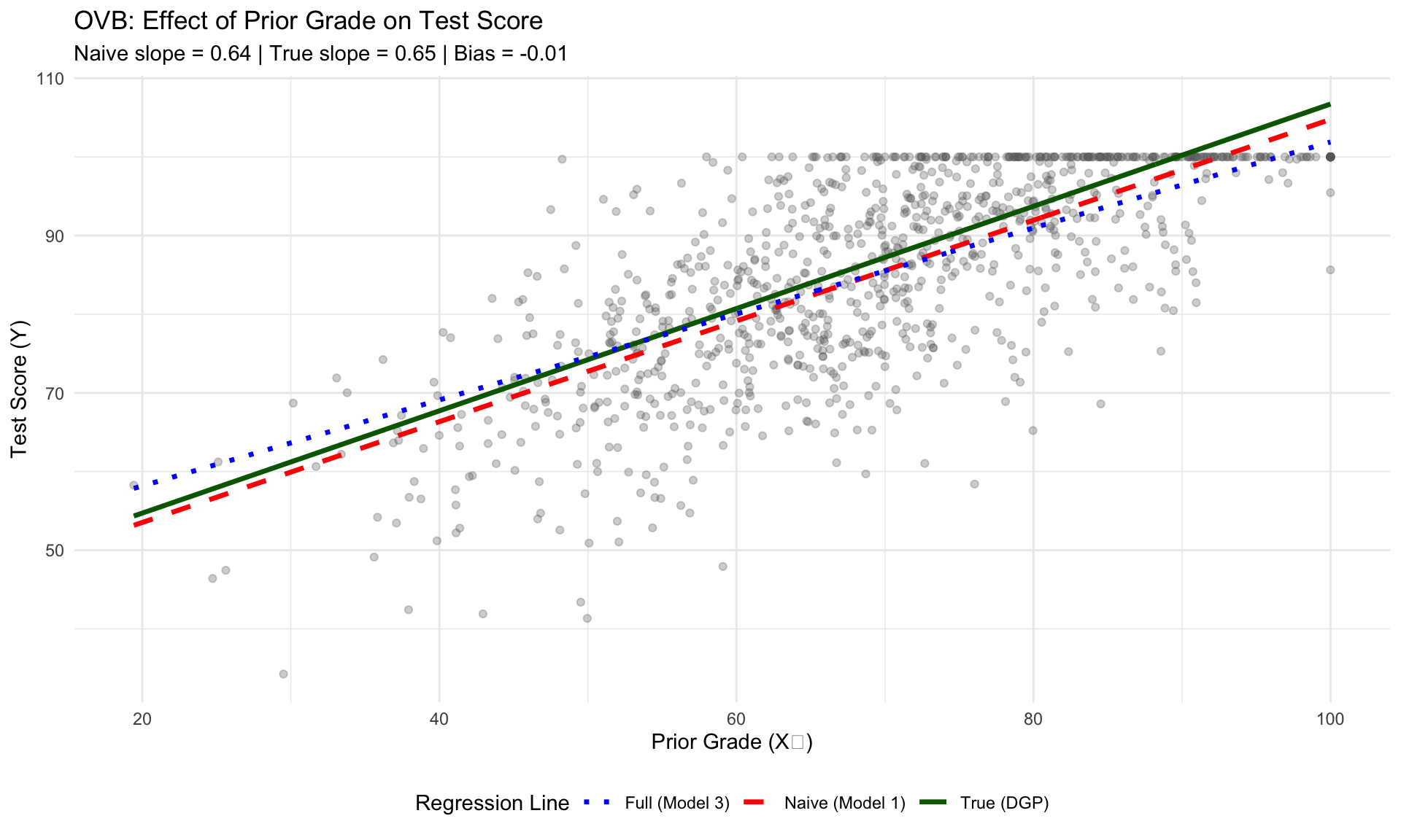
Show code
mean_prior <- mean(data$prior_grade)

data$true_fitted_x2 <- true_beta_0 + true_beta_1 * mean_prior + true_beta_2 * data$study_hours
data$naive_fitted_x2 <- predict(model_2, data)
data$full_fitted_x2 <- coef(model_3)[1] + coef(model_3)[2] * mean_prior + coef(model_3)[3] * data$study_hours

ggplot(data, aes(x = study_hours, y = test_score)) +
  geom_point(alpha = 0.3, color = "gray40") +
  geom_line(aes(y = true_fitted_x2, color = "True (DGP)"), linewidth = 1.2) +
  geom_line(aes(y = naive_fitted_x2, color = "Naive (Model 2)"), linewidth = 1.2, linetype = "dashed") +
  geom_line(aes(y = full_fitted_x2, color = "Full (Model 3)"), linewidth = 1.2, linetype = "dotted") +
  scale_color_manual(values = c("True (DGP)" = "darkgreen",
                                 "Naive (Model 2)" = "red",
                                 "Full (Model 3)" = "blue")) +
  labs(x = "Study Hours per Week (X₂)",
       y = "Test Score (Y)",
       title = "OVB: Effect of Study Hours on Test Score",
       subtitle = paste0("Naive slope = ", round(coef(model_2)[2], 3),
                        " | True slope = ", true_beta_2,
                        " | Bias = ", round(coef(model_2)[2] - true_beta_2, 3)),
       color = "Regression Line") +
  theme_minimal() +
  theme(legend.position = "bottom")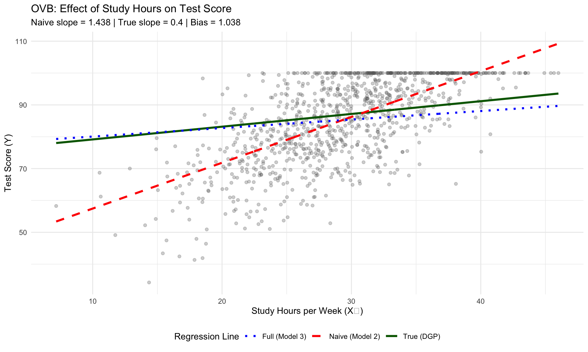
4.1.6 Summary: The Direction of OVB
The sign of the omitted variable bias depends on two things:
- The sign of the omitted variable’s true coefficient (\(\beta\))
- The sign of the correlation between the included and omitted variables
| Sign of \(\beta\) | Sign of Corr(\(X_{included}\), \(X_{omitted}\)) | Direction of Bias |
|---|---|---|
| + | + | Positive (overestimate) |
| + | - | Negative (underestimate) |
| - | + | Negative (underestimate) |
| - | - | Positive (overestimate) |
In our example, both \(\beta_1\) and \(\beta_2\) are positive, and \(X_1\) and \(X_2\) are positively correlated. Therefore, omitting either variable leads to positive bias (overestimation) of the remaining coefficient.
NoteA Great Exercise
Solidify this concept for yourself is to think of a situation that is clear to you for each of the other three cases.
Show code
summary_df <- data.frame(
  Model = c("Model 1 (X₁ only)", "Model 2 (X₂ only)"),
  Omitted_Variable = c("Study Hours (X₂)", "Prior Grade (X₁)"),
  Included_Coef_Estimate = c(round(coef(model_1)[2], 4), round(coef(model_2)[2], 4)),
  True_Value = c(true_beta_1, true_beta_2),
  Bias = c(round(coef(model_1)[2] - true_beta_1, 4), round(coef(model_2)[2] - true_beta_2, 4)),
  Bias_Direction = c("Positive (overestimate)", "Positive (overestimate)")
)

knitr::kable(summary_df,
             col.names = c("Model", "Omitted Variable", "Estimate", "True Value", "Bias", "Direction"),
caption = "Summary of OVB in each misspecified model")| Model | Omitted Variable | Estimate | True Value | Bias | Direction | |
|---|---|---|---|---|---|---|
| prior_grade | Model 1 (X₁ only) | Study Hours (X₂) | 0.6404 | 0.65 | -0.0096 | Positive (overestimate) |
| study_hours | Model 2 (X₂ only) | Prior Grade (X₁) | 1.4384 | 0.40 | 1.0384 | Positive (overestimate) |
TipWhat’s next?
When a regressor is measured with error instead of omitted entirely, see Measurement Error. For the instrumental variables solution to endogeneity, see Instrumental Variables. For panel data approaches, see Fixed Effects.
A reminder that there is nothing “Simple” about “Simple Linear Regression”. It’s merely the terminology from the text. It’s also important to note that the order of these assumptions is slightly different from chapter 2: SR1 ↔︎ RS1, SR2 ↔︎ RS3: Both are exogeneity, but SR2 is stricter (conditions on all (x)); RS3 conditions only on (x_i). SR3 ↔︎ RS4, SR4 ↔︎ RS2, SR5 ↔︎ RS5, SR6 ↔︎ RS6.↩︎