7 Simultaneous Equations

Identification and Estimation When Causation Runs Both Ways

Simultaneous Equations

Identification

2SLS

Author

Jake Anderson

Published

March 3, 2026

Modified

March 4, 2026

This chapter deals with what happens when two or more variables are determined together at the same time.

7.1 Motivation

In most regressions, we think of $x$ as causing $y$. But sometimes causation runs both ways simultaneously. Think about supply and demand at a farmers’ market. The price of strawberries depends on how many people want them (demand) and how many farmers brought them (supply). But the quantity sold also depends on the price. So price determines quantity, and quantity determines price — they settle together in equilibrium.

When we observe price and quantity data from a market, each data point is an equilibrium — the intersection of supply and demand. If we just run OLS of $Q$ on $P$, we don’t recover the demand curve or the supply curve. We get some confused mixture of both.

7.2 Worked Example: Bruin Boba

7.2.1 Supply and Demand at Bruin Boba

Imagine you track weekly price per cup ($P_t$) and cups sold ($Q_t$) at Bruin Boba:

Week 1 (normal): Nothing special.
Week 2 (hot week): It’s 90°F all week $\implies$ lots more students want boba (demand shifts out).
Week 3 (pearl shortage): Tapioca pearls get expensive $\implies$ higher costs (supply shifts in).
Week 4 (Instagram post): Bruin Boba goes semi-viral $\implies$ more customers (demand shifts out).
Week 5 (milk price spike): Milk cost jumps $\implies$ higher costs (supply shifts in).

Your dataset is just equilibrium points $(P_t, Q_t)$ generated by different shocks.

7.2.2 The True Demand and Supply

Let the true (linear) curves be:

\[ \textbf{Demand:}\quad Q = 200 - 20P + u_D \tag{7.1}\]

\[ \textbf{Supply:}\quad Q = -40 + 30P + v_S \tag{7.2}\]

where $u_D$ is a demand shifter (hot weather, virality, etc.) and $v_S$ is a supply shifter (input costs). When input costs rise, supply shifts left, which we model as negative $v_S$.

7.2.3 Weekly Shocks and Equilibrium Outcomes

Week	Story Shock	$(u_D, v_S)$	Price ($P^*$)	Cups Sold ($Q^*$)
1	Normal	$(0, 0)$	$4.80	104
2	Hot week (demand up)	$(60, 0)$	$6.00	140
3	Pearl shortage (cost up)	$(0, -60)$	$6.00	80
4	Instagram (demand up)	$(40, 0)$	$5.60	128
5	Milk spike (cost up)	$(0, -80)$	$6.40	72

7.2.4 Solving for Equilibrium

Equilibrium satisfies demand = supply:

\[ 200 - 20P + u_D = -40 + 30P + v_S \]

\[ 240 + u_D - v_S = 50P \quad\Rightarrow\quad P^* = \frac{240 + u_D - v_S}{50} \]

Then plug into demand to get $Q^*$:

\[ Q^* = 200 - 20P^* + u_D \]

Show code

# Bruin Boba: structural model + equilibrium points
df <- data.frame(
  week = c("W1 normal", "W2 hot (demand+)", "W3 pearls costly (supply-)",
           "W4 Instagram (demand+)", "W5 milk costly (supply-)"),
  uD = c(0, 60, 0, 40, 0),
  vS = c(0, 0, -60, 0, -80)
)

# Equilibrium solver
df$P <- (240 + df$uD - df$vS) / 50
df$Q <- 200 - 20*df$P + df$uD

knitr::kable(df[, c("week", "uD", "vS", "P", "Q")],
             col.names = c("Week", "u_D", "v_S", "P*", "Q*"),
             caption = "Equilibrium outcomes for each week")

Equilibrium outcomes for each week
Week	u_D	v_S	P*	Q*
W1 normal	0	0	4.8	104
W2 hot (demand+)	60	0	6.0	140
W3 pearls costly (supply-)	0	-60	6.0	80
W4 Instagram (demand+)	40	0	5.6	128
W5 milk costly (supply-)	0	-80	6.4	72

Warning

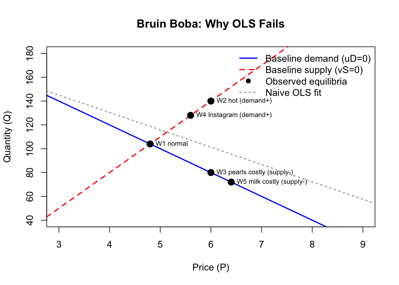
Week 2 and Week 3 have the same price ($P=6.0$) but very different quantities (140 vs 80) because one week is a demand shift and the other is a supply shift. A single OLS line through $(P_t, Q_t)$ can’t recover demand (or supply).

7.2.5 Visualizing the Problem

Show code

# Price grid for plotting baseline curves
Pgrid <- seq(0, 10, by = 0.05)
Qd0 <- 200 - 20*Pgrid          # baseline demand (uD=0)
Qs0 <- -40 + 30*Pgrid          # baseline supply (vS=0)

# Plot baseline demand and supply
plot(Pgrid, Qd0, type = "l", col = "blue", lwd = 2,
     xlab = "Price (P)", ylab = "Quantity (Q)",
     xlim = c(3, 9), ylim = c(40, 180),
     main = "Bruin Boba: Why OLS Fails")
lines(Pgrid, Qs0, lty = 2, col = "red", lwd = 2)

# Add equilibrium data points
points(df$P, df$Q, pch = 19, cex = 1.5)
text(df$P, df$Q, labels = df$week, pos = 4, cex = 0.7)

# Add naive OLS line
ols_fit <- lm(Q ~ P, data = df)
abline(ols_fit, col = "darkgray", lwd = 2, lty = 3)

legend("topright",
       legend = c("Baseline demand (uD=0)", "Baseline supply (vS=0)",
                  "Observed equilibria", "Naive OLS fit"),
       lty = c(1, 2, NA, 3), lwd = c(2, 2, NA, 2),
       pch = c(NA, NA, 19, NA),
       col = c("blue", "red", "black", "darkgray"),
       bty = "n")

Equilibrium points from shifting demand and supply curves

The gray dashed line shows what OLS estimates when you naively regress $Q$ on $P$. It doesn’t match the true demand curve (blue) or the supply curve (red). This is simultaneity bias: because $P$ and $Q$ are jointly determined in equilibrium, $\text{Cov}(P, u_D) \neq 0$ and OLS is biased and inconsistent.

Note

To estimate demand, we need an instrumental variable that shifts supply (like input costs) but is uncorrelated with demand shocks. This isolates movement along the demand curve rather than shifts of it.

7.3 Structural Equations

The structural form describes the behavioral relationships — what economic theory says about how agents make decisions.

Consider the truffle market:

\[ \text{Demand:} \quad Q = \alpha_1 + \alpha_2 P + \alpha_3 PS + \alpha_4 DI + e^d \tag{7.3}\]

\[ \text{Supply:} \quad Q = \beta_1 + \beta_2 P + \beta_3 PF + e^s \tag{7.4}\]

where:

$P$ = price of truffles, $Q$ = quantity of truffles
$PS$ = price of a substitute good (exogenous)
$DI$ = disposable income of consumers (exogenous)
$PF$ = price of a factor of production (exogenous)
$e^d, e^s$ = demand and supply shocks

Endogenous variables ($P$ and $Q$): determined within the system by the intersection of supply and demand. Their values depend on the shocks $e^d$ and $e^s$.

Exogenous variables ($PS$, $DI$, $PF$): determined outside the system. They shift the curves but are not affected by the market equilibrium.

Notice that in the demand equation, $P$ is endogenous — it’s correlated with $e^d$ because supply shocks (which affect $P$ through equilibrium) are baked into the error. OLS requires $\text{Cov}(P, e^d) = 0$, but here $\text{Cov}(P, e^d) \neq 0$. So OLS on the structural equations is biased and inconsistent — the same endogeneity problem we saw in the IV chapter.

7.4 Reduced-Form Equations

The reduced form expresses each endogenous variable as a function of only exogenous variables. We get these by solving the structural system.

Derivation: Set demand equal to supply:

\[ \alpha_1 + \alpha_2 P + \alpha_3 PS + \alpha_4 DI + e^d = \beta_1 + \beta_2 P + \beta_3 PF + e^s \]

Solve for $P$:

\[ (\alpha_2 - \beta_2) P = (\beta_1 - \alpha_1) - \alpha_3 PS - \alpha_4 DI + \beta_3 PF + (e^s - e^d) \]

\[ P = \frac{\beta_1 - \alpha_1}{\alpha_2 - \beta_2} - \frac{\alpha_3}{\alpha_2 - \beta_2} PS - \frac{\alpha_4}{\alpha_2 - \beta_2} DI + \frac{\beta_3}{\alpha_2 - \beta_2} PF + \frac{e^s - e^d}{\alpha_2 - \beta_2} \tag{7.5}\]

This can be written compactly as:

\[ P = \pi_{10} + \pi_{11} PS + \pi_{12} DI + \pi_{13} PF + v_1 \]

Similarly, substituting back gives the reduced form for $Q$:

\[ Q = \pi_{20} + \pi_{21} PS + \pi_{22} DI + \pi_{23} PF + v_2 \]

The nice thing about reduced forms is that OLS actually works on them — the right-hand side has only exogenous variables, so there’s no endogeneity problem. These reduced-form equations are exactly the first-stage regressions in 2SLS. The reduced-form parameters ($\pi$’s) are combinations of structural parameters ($\alpha$’s and $\beta$’s).

Think: For a simpler model where Demand is $Q = \alpha_1 P + \alpha_2 X + e^d$ and Supply is $Q = \beta_1 P + e^s$, derive the reduced form for $P$.

Set demand = supply: $\alpha_1 P + \alpha_2 X + e^d = \beta_1 P + e^s$

\[(\alpha_1 - \beta_1)P = -\alpha_2 X + (e^s - e^d)\]

\[P = \frac{-\alpha_2}{\alpha_1 - \beta_1} X + \frac{e^s - e^d}{\alpha_1 - \beta_1} = \frac{\alpha_2}{\beta_1 - \alpha_1} X + \frac{e^d - e^s}{\beta_1 - \alpha_1}\]

This is the reduced form: $P = \pi_1 X + v_1$ where $\pi_1 = \alpha_2 / (\beta_1 - \alpha_1)$.

7.5 The Identification Problem

So can we actually recover the structural parameters? This depends on whether the equations are identified.

7.5.1 The Order Condition

In a system of $M$ simultaneous equations, an equation is identified if it excludes at least $M - 1$ variables that appear elsewhere in the system.

Intuition: To trace out the demand curve, we need something that shifts supply but not demand. If supply shifts while demand stays fixed, the equilibrium moves along the demand curve, revealing its slope.

Checking the truffle model:

Demand equation (Equation 7.3): $PF$ is excluded (it’s in supply but not demand). One exclusion $\geq M - 1 = 1$. $\checkmark$ Identified.
Supply equation (Equation 7.4): $PS$ and $DI$ are excluded (they’re in demand but not supply). Two exclusions $\geq M - 1 = 1$. $\checkmark$ Identified (actually overidentified — more exclusions than needed).

Think: What if both equations contained all the same variables?

Then neither equation would exclude anything. We’d have zero exclusions, which is less than $M - 1 = 1$. Both equations would be unidentified — no estimation method can recover the structural parameters. This is the original supply-and-demand identification problem: without shifters, you can’t tell the curves apart.

7.6 2SLS for Simultaneous Systems

Once we know an equation is identified, we estimate it with two-stage least squares — same method as the IV chapter, just applied to each structural equation separately.

Estimating the demand equation:

First stage: Regress $P$ on all exogenous variables ($PS$, $DI$, $PF$) to get $\hat{P}$
Second stage: In the demand equation, replace $P$ with $\hat{P}$ and estimate by OLS

The instruments for $P$ in the demand equation are the variables excluded from demand — here, $PF$ (the supply shifter).

Estimating the supply equation:

First stage: Same regression — $P$ on all exogenous variables
Second stage: In the supply equation, replace $P$ with $\hat{P}$

The instruments for $P$ in the supply equation are $PS$ and $DI$ (the demand shifters).

Same rule as in the IV chapter: check that the instruments are strong. The F-statistic from the first-stage regression should exceed 10 (Staiger-Stock rule of thumb). Weak instruments lead to biased and imprecise 2SLS estimates here too.

8 Example: The Truffle Market

The truffle market model:

\[\text{Demand:} \quad Q = \alpha_1 + \alpha_2 P + \alpha_3 PS + \alpha_4 DI + e^d\] \[\text{Supply:} \quad Q = \beta_1 + \beta_2 P + \beta_3 PF + e^s\]

(a) Which variables are endogenous and which are exogenous?

Answer

Endogenous: $P$ and $Q$ — jointly determined by the intersection of supply and demand.

Exogenous: $PS$ (price of substitute), $DI$ (disposable income), $PF$ (price of factor of production) — determined outside the truffle market.

(b) Check identification for both equations.

Answer

With $M = 2$ equations, we need at least $M - 1 = 1$ exclusion per equation.

Demand: Excludes $PF$ (1 exclusion $\geq 1$). $\checkmark$ Just identified.
Supply: Excludes $PS$ and $DI$ (2 exclusions $\geq 1$). $\checkmark$ Overidentified.

(c) A researcher naively runs OLS on the demand equation and gets $\hat{\alpha}_2 = -0.37$. The 2SLS estimate is $\hat{\alpha}_2 = -0.53$. Why are they different, and which should we trust?

Answer

They differ because OLS is biased and inconsistent — $P$ is endogenous, so $\text{Cov}(P, e^d) \neq 0$. The OLS estimate of $-0.37$ understates the true price sensitivity of demand (it’s biased toward zero because of simultaneity).

We should trust the 2SLS estimate ($-0.53$), which uses $PF$ as an instrument for $P$. Since $PF$ shifts supply but not demand, it isolates movement along the demand curve. Assuming the instrument is valid and strong, 2SLS is consistent.

(d) For the supply equation, a Sargan overidentification test gives $NR^2 = 0.43$ with 1 degree of freedom. The 5% critical value for $\chi^2_1$ is 3.84. Interpret.

Answer

$H_0$: All surplus instruments are valid (uncorrelated with $e^s$).

Since $0.43 < 3.84$, we fail to reject $H_0$. The surplus instrument appears valid.

Note: The supply equation has $L = 2$ instruments ($PS$ and $DI$) for $B = 1$ endogenous variable ($P$), so $L - B = 1$ surplus instrument can be tested.

8.1 Slide Deck

Download slides (PDF)

Download presentation slides (with transitions) (PDF)

What’s next?

The identification logic from simultaneous equations reappears in Instrumental Variables. For panel data versions of these ideas, see Panel Data.