9 Fixed Effects
Group-Specific Intercepts and the Within Estimator
A running example with two athletic teams shows why pooled OLS swings between wildly different slope estimates depending on group composition, even when the true effect is the same. Map the problem to the omitted-variable-bias framework, watch the slope estimate move as the scenario changes, then introduce fixed effects as a structural fix: give every group its own intercept. End with the within estimator (demeaning), the equivalence to LSDV, and the rank condition that constrains identification.
9.1 The Setup
A coach is studying whether more training hours produce better performance. The data set is straightforward: for each athlete, the number of training hours over the season and an end-of-season performance score. The coach plans to run a simple linear regression and report the slope.
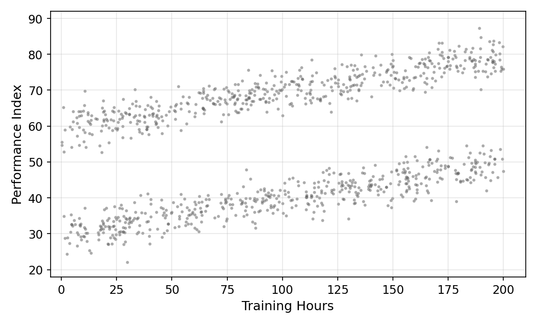
The twist is that the athletes belong to two teams: Junior Varsity (JV) and Varsity. They share the same training program but enter the season with very different skill levels. Assume the truth is:
- JV players start at a baseline of 30 performance points.
- Varsity players start at a baseline of 60.
- Every athlete, regardless of team, gains 1 performance point for every 10 additional training hours. So the true slope is \(\beta_1 = 0.1\) and it’s the same for both groups.
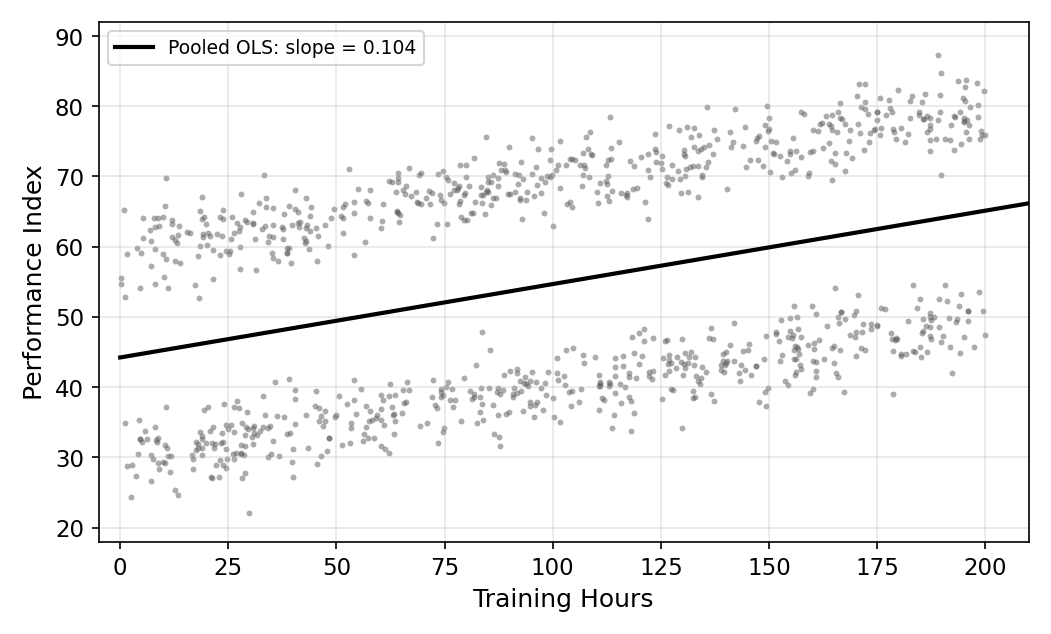
If we don’t tell the coach about the two teams, the model they would fit is
\[ \text{Performance}_i = \beta_0 + \beta_1 \, \text{Hours}_i + \varepsilon_i. \tag{9.1}\]
One intercept for everyone. JV’s true baseline is 30 and Varsity’s is 60. One intercept cannot be right for both groups. Something is going to give, and the question is what, depending on the data we feed in.
The pooled OLS model in Equation 9.1 is what you fit when you ignore group structure. It is the natural first thing to try, and we will see exactly when it works (rarely) and when it fails (often).
9.2 When Pooled OLS Looks Fine
Suppose the JV and Varsity samples are perfectly balanced (50/50) and both groups have the same average training hours. The pooled OLS slope comes out at roughly \(\hat\beta_1 = 0.10\), matching the true slope. Looks good. Case closed?
No. Pooled OLS was right by accident. With balanced sampling and identical \(x\) distributions across groups, the bias terms cancel and OLS happens to land on the truth. The moment either of those conditions breaks, different group sizes, different \(x\) distributions, pooled OLS goes off the rails. The next two sections each break exactly one of them.
9.3 When the Training Distribution Differs Across Groups
Real teams aren’t symmetric. Some teams push harder, some are catching up, some have access to better facilities. So in practice the training-hours distribution often differs across groups. That single difference is enough to break pooled OLS.
Scenario A: Varsity trains more. Suppose Varsity players average more hours than JV players. (Maybe they’re more competitive, or their coach drives them harder.) Pooled OLS sees: athletes at the top of the training-hours distribution have very high performance, and athletes at the bottom have low performance. It happily fits a steep line.
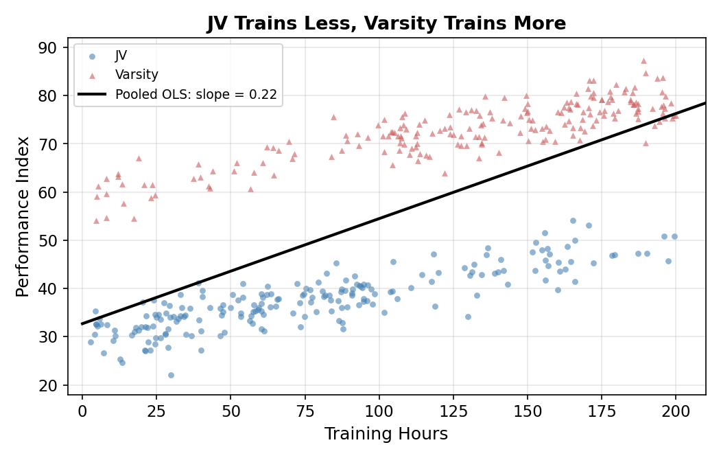
The result: \(\hat\beta_1 \approx 0.22\). The true slope is \(0.10\), so OLS more than doubles the return to training.
Scenario B: JV trains more (catching up). Now flip it. JV players are the ones putting in extra hours, maybe to close the gap. The high-training observations now sit on the JV line (lower baseline), and the low-training observations sit on the Varsity line (higher baseline). Pooled OLS fits a nearly-flat line through this configuration.
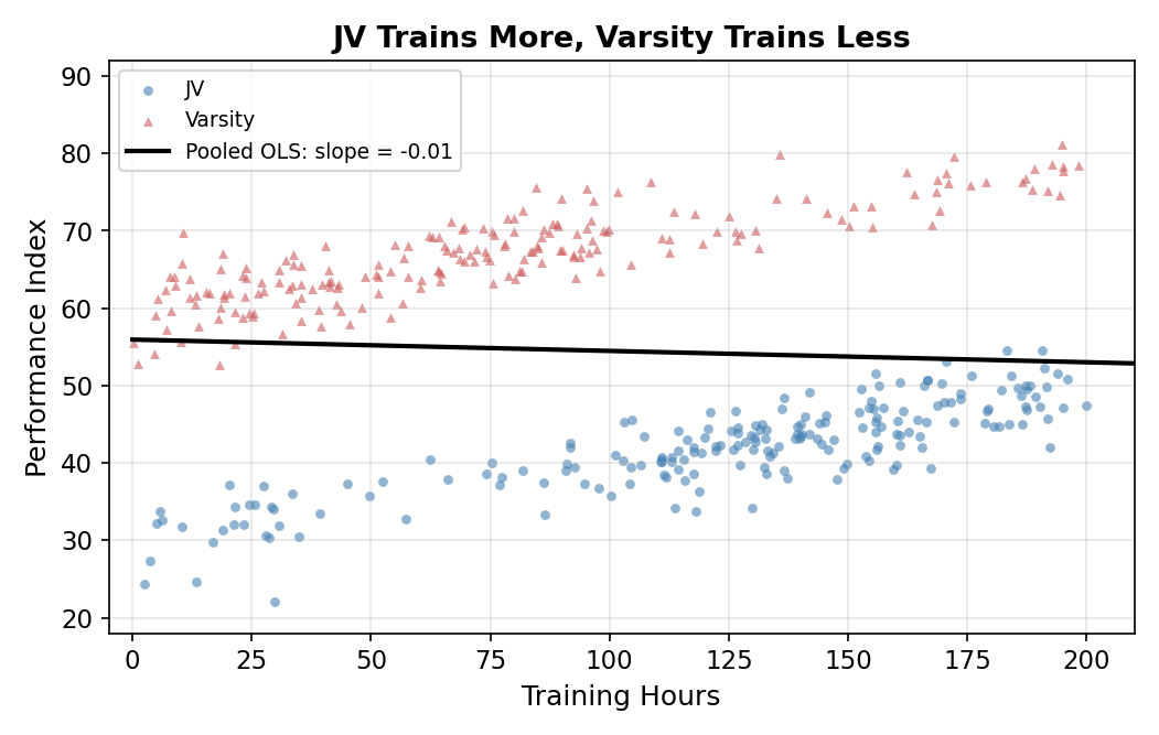
The result: \(\hat\beta_1 \approx -0.02\). The true slope is \(0.10\), and OLS reports essentially no effect of training, even slightly negative.
Same data-generating process. Same true slope. The OLS estimate just swung from \(-0.02\) to \(+0.22\) depending on which team trains more. That is not a small effect.
9.3.1 Mapping This to Omitted Variable Bias
What we just walked through is omitted-variable bias in panel form. The “omitted variable” is group membership. Recall the OVB framework from the OVB chapter:
- Short regression (what we ran, omitting group): \(y_i = \beta_0 + \beta_1 x_{1i} + u_i\)
- Long regression (with group included): \(y_i = \beta_0 + \beta_1 x_{1i} + \beta_2 x_{2i} + \varepsilon_i\), where \(x_{2i}\) is a group dummy
- Auxiliary regression (group on training): \(x_{2i} = \delta_0 + \delta_1 x_{1i} + v_i\)
The OVB formula tells us how short and long estimates differ:
\[ \hat\beta_1^{\text{short}} = \hat\beta_1^{\text{long}} + \hat\beta_2 \cdot \hat\delta_1. \tag{9.2}\]
For our training example, \(\hat\beta_2\) is the effect of being Varsity on performance, holding training fixed, that’s the baseline gap of about 30 points, so \(\hat\beta_2 > 0\). The bias direction is then determined by \(\hat\delta_1\), the auxiliary slope of group on training.
| Scenario | \(\hat\delta_1\) (group on training) | Bias \(\hat\beta_2 \cdot \hat\delta_1\) | OLS slope |
|---|---|---|---|
| Varsity trains more | \(> 0\) | \(+\) | 0.22 |
| Equal training | \(\approx 0\) | \(\approx 0\) | 0.10 |
| JV trains more | \(< 0\) | \(-\) | \(-0.02\) |
The middle column is just the OVB formula playing out: positive \(\hat\delta_1\) gives positive bias (Varsity case), negative \(\hat\delta_1\) gives negative bias (JV case). The OLS slope is the true effect plus that bias.
It depends on whether 200 hours puts them on the JV portion or the Varsity portion of the data, and on the slope OLS estimated:
- Scenario A (Varsity trains more, \(\hat\beta_1 = 0.22\)): if Varsity averages around 250 hours and JV around 150, then 200 is in between. OLS predicts roughly \(\hat\beta_0 + 0.22 \times 200\), but the OLS intercept here is also tilted, so the prediction is in the upper range. The OLS line goes too steeply through the data.
- Scenario B (JV trains more, \(\hat\beta_1 \approx 0\)): OLS predicts essentially the average performance across both teams regardless of training. The pooled line is roughly flat.
The same 200 hours produces wildly different predictions across scenarios, even though the true effect of those 200 hours is identical: \(0.1 \times 200 = 20\) extra performance points on top of the athlete’s team baseline.
9.4 When the Sample Composition Is Imbalanced
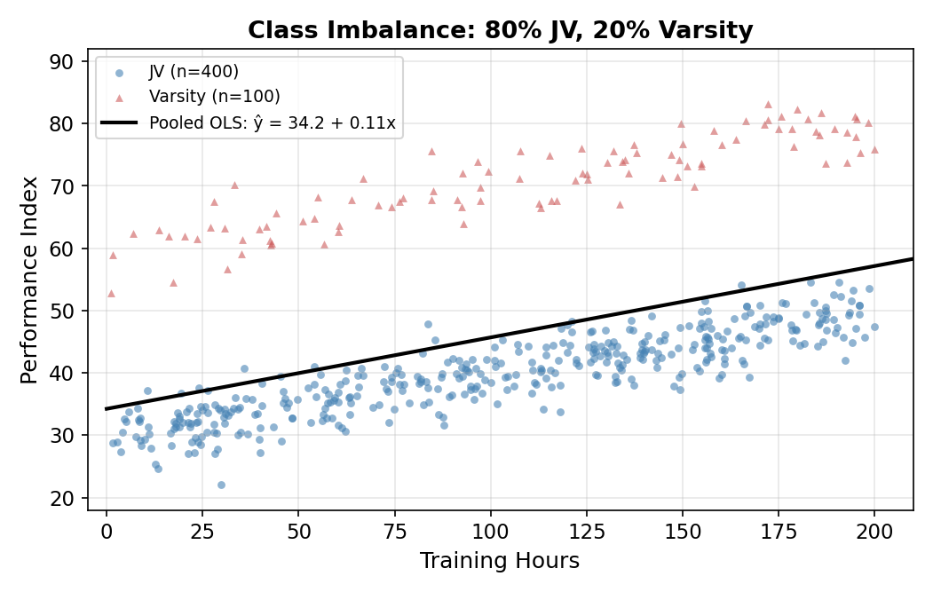
Now suppose the training distribution is the same across groups (Scenario from Section 9.2) but the sample is no longer 50/50. With 80% JV and 20% Varsity, the OLS intercept is a weighted average of the two group baselines:
\[ \hat\beta_0 = \frac{n_{\text{JV}}}{n} \cdot \beta_{0,\text{JV}} + \frac{n_{\text{Var}}}{n} \cdot \beta_{0,\text{Var}}. \tag{9.3}\]
With 80% JV, the weighted average is \(0.8(30) + 0.2(60) = 36\). The OLS intercept comes out near 34 (small adjustment for the data fit). It’s close to JV’s true intercept of 30 but quite far from Varsity’s 60. Predictions for Varsity players are systematically low by about 26 points.
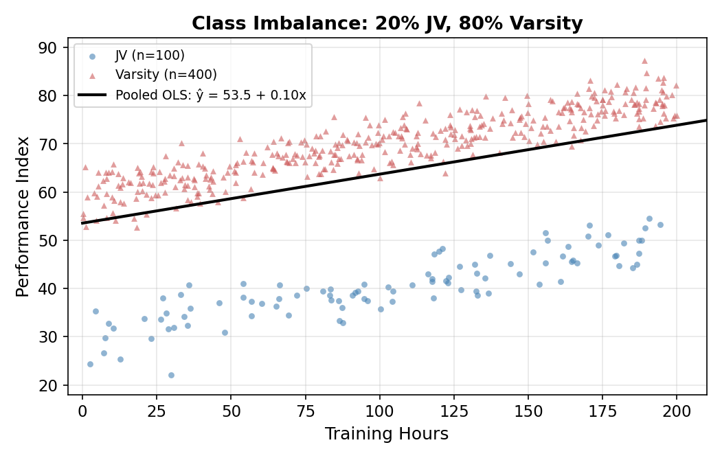
Flip the imbalance to 20% JV and 80% Varsity: the OLS intercept is \(0.2(30) + 0.8(60) = 54\). Now JV predictions are off by 24 points in the other direction.
| Sample composition | OLS intercept | JV true (30) | Varsity true (60) |
|---|---|---|---|
| 80% JV / 20% Varsity | 34 | close | off by 26 |
| 50% / 50% | 44 | off by 14 | off by 16 |
| 20% JV / 80% Varsity | 54 | off by 24 | close |
The slope is approximately correct in each row, but a single intercept cannot serve both groups. The error is large for whichever group is the minority. And the researcher often doesn’t control sample composition, it’s just whatever the data happens to be.
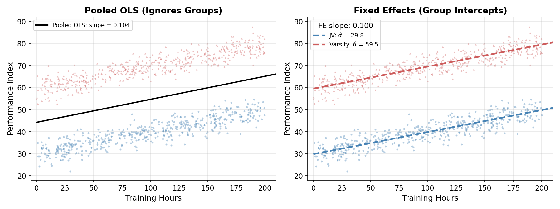
The lesson from the last two sections: pooled OLS uses one intercept where the data has two. Sometimes it gets lucky on the slope (balanced sample, similar \(x\) distribution); sometimes it doesn’t. The structural fix is to stop forcing one intercept on data that has two.
9.5 Fixed Effects: A Separate Intercept per Group
Every problem above stems from a single architectural choice: forcing one baseline (\(\beta_0\)) on data with multiple group baselines (\(\beta_{0,\text{JV}}\), \(\beta_{0,\text{Var}}\), more generally \(\alpha_j\) for group \(j\)). The fix is to let each group have its own intercept:
\[ y_{ij} = \alpha_j + \beta \, x_{ij} + \varepsilon_{ij}. \tag{9.4}\]
The subscript \(j\) on the intercept does all the work. Instead of one number shared by everyone, \(\alpha_j\) is a different number for each group. This is the fixed effects model.
Equivalently, write it with explicit dummies for each group:
\[ y_i = \beta \, x_i + \alpha_{\text{JV}} \cdot \mathbb{1}\{i \in \text{JV}\} + \alpha_{\text{Var}} \cdot \mathbb{1}\{i \in \text{Var}\} + \varepsilon_i. \]
There is no overall intercept here, just one intercept per group. This formulation is called Least Squares Dummy Variables (LSDV). It is conceptually clean: include a dummy for every group, fit OLS, read off the group baselines and the single slope.
The estimated slope under FE recovers the true value:
\[ \hat\beta^{\text{FE}} = 0.100 \quad (\text{true} = 0.10). \]
The estimated intercepts pin down each group’s baseline: \(\hat\alpha_{\text{JV}} = 29.8\) (true 30) and \(\hat\alpha_{\text{Var}} = 59.5\) (true 60). The estimator gets the slope right because it asks within each group: among JV players, do those who train more perform better? Among Varsity players, do those who train more perform better? It pools the within-group answers and ignores everything that varies between groups.
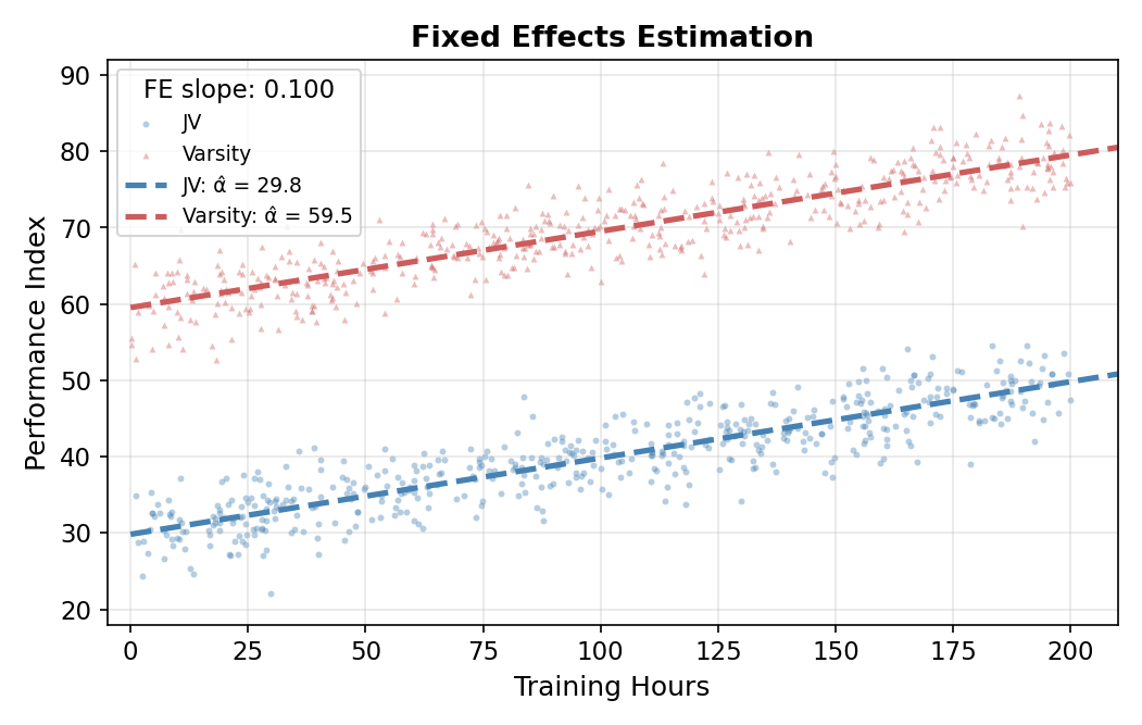
The figure makes the within-group identification visible. FE doesn’t draw one line through both clouds; it draws two parallel lines, one anchored at each team’s baseline, sharing a single slope. The two lines are parallel because the slope is the same for both groups by assumption (the same return to training applies everywhere). What FE learns from the data is where each line sits vertically (the intercepts) and how steep they are (the shared slope).
Within variation is variation in \(x\) around the group mean \(\bar x_j\). Between variation is variation across group means \(\bar x_j\). FE uses only the within piece.
The within-group identification strategy is what makes FE robust. As long as \(x\) varies within each group (each team has athletes with different training hours), the slope is identified. The between-group differences in average \(x\), which were the source of the bias above, are absorbed into the group intercepts and don’t affect the slope.
9.5.1 The Rank Condition
FE has one more constraint than pooled OLS. The basic identification rule is “you need at least two points to draw a line” (one intercept + one slope = two unknowns). Pooled OLS needs two observations total. FE with \(J\) groups has \(J + 1\) unknowns (\(J\) intercepts + one slope), so you need at least two observations per group. If a group has only one observation, its intercept absorbs the entire fit and the slope contribution from that group is zero.
For our two-team example: \(J = 2\) groups, so \(J + 1 = 3\) unknowns. Minimum data: 2 JV + 2 Varsity = 4 observations. In a typical 500-athlete panel that’s not a binding constraint. But in panels with many groups and short time series, the rank condition can quietly bite.
9.6 Connection to Panel Data
The “training hours by team” example maps directly to the panel-data setup that fills the rest of the chapter. Replace “team” with “unit” (which could be individual, firm, country, hospital) and “training hours” with whatever time-varying regressor you care about. Add a time subscript \(t\):
\[ y_{it} = \alpha_i + \beta \, x_{it} + \varepsilon_{it}. \tag{9.5}\]
The \(\alpha_i\) is an individual fixed effect, unit \(i\)’s permanent unobserved level, absorbing everything that’s constant within \(i\) but varies across \(i\)’s. That’s a lot: unobserved ability, firm management quality, country-level institutions, hospital protocols. Anything that doesn’t change for unit \(i\) across the periods in your sample is wrapped into \(\alpha_i\).
Two practical examples of what an FE specification controls for “for free”:
- Wages and education. A worker’s unobserved ability is constant. FE on a wage panel sweeps it out, so the OLS-style ability bias from the IV chapter goes away.
- Firm productivity. Unobserved management quality is constant for a given firm. FE on a firm-level panel controls for it without ever observing it directly.
The cost is also worth flagging: anything else that doesn’t change for unit \(i\) gets absorbed too, including things you might want to estimate. We come back to this when we discuss random effects and the Hausman-Taylor estimator.
9.7 Estimating FE Two Ways
There are two equivalent ways to estimate the FE model. They produce identical \(\hat\beta\).
9.7.1 Method 1: Least Squares Dummy Variables (LSDV)
Add a dummy for each unit and run OLS:
\[ y_{it} = \beta \, x_{it} + \sum_i \alpha_i D_i + \varepsilon_{it}. \tag{9.6}\]
That’s literally just OLS with \(N\) dummies on the right-hand side. Software handles it. The output is the slope \(\hat\beta\) and a long list of unit-specific intercepts \(\hat\alpha_1, \ldots, \hat\alpha_N\). With 5 units, that’s a clean table. With 5,000 units it is unwieldy but computationally fine.
9.7.2 Method 2: The Within Estimator (Demeaning)
The elegant alternative is to demean the data and run OLS on the deviations. The walkthrough below builds it from scratch.
Step 1, Average the model within each unit. Start with Equation 9.5 and take the time mean of both sides:
\[ \bar y_i = \alpha_i + \beta \, \bar x_i + \bar\varepsilon_i, \tag{9.7}\]
where \(\bar y_i = \tfrac{1}{T} \sum_t y_{it}\) (and similarly for \(\bar x_i\), \(\bar\varepsilon_i\)). Notice that \(\alpha_i\) survives the averaging because it doesn’t vary across \(t\), averaging a constant gives back the constant.
Step 2, Subtract the unit mean from the original equation. Subtract Equation 9.7 from Equation 9.5:
\[ (y_{it} - \bar y_i) = (\alpha_i - \alpha_i) + \beta\,(x_{it} - \bar x_i) + (\varepsilon_{it} - \bar\varepsilon_i). \]
The fixed effect cancels. Define the demeaned variables \(\ddot y_{it} = y_{it} - \bar y_i\) and \(\ddot x_{it} = x_{it} - \bar x_i\):
\[ \ddot y_{it} = \beta \, \ddot x_{it} + \ddot\varepsilon_{it}. \tag{9.8}\]
That’s a simple regression with no intercept and no fixed effects. Just run OLS on it.
Step 3, Compute \(\hat\beta\).
\[ \hat\beta^{\text{within}} = \frac{\sum_i \sum_t (x_{it} - \bar x_i)(y_{it} - \bar y_i)}{\sum_i \sum_t (x_{it} - \bar x_i)^2}. \tag{9.9}\]
This is the within estimator. It uses only within-unit variation, each athlete’s deviation from their team’s average training, and their deviation from the team’s average performance.
9.7.3 Why Demeaning Doesn’t Throw Out Useful Information
It looks suspicious that we just subtracted off the mean and lost (potentially) most of the variation in \(x\). The reassuring fact is that demeaning doesn’t change the relevant covariance. Let \(c_i = \bar x_i\) and \(d_i = \bar y_i\) be the unit-level means (constants within each unit). Then
\[ \operatorname{Cov}(x_{it} - c_i,\; y_{it} - d_i) = \operatorname{Cov}(x_{it}, y_{it}) - \operatorname{Cov}(x_{it}, d_i) - \operatorname{Cov}(c_i, y_{it}) + \operatorname{Cov}(c_i, d_i). \]
Within each unit, \(c_i\) and \(d_i\) are constants. The covariance of any random variable with a constant is zero, so the three subtracted terms vanish and we are left with
\[ \operatorname{Cov}(x_{it} - \bar x_i,\; y_{it} - \bar y_i) = \operatorname{Cov}(x_{it}, y_{it}). \]
So the demeaned covariance equals the original covariance. The information about the slope is intact; the only thing demeaning removes is the systematic between-unit level differences, which were the source of the bias.
When \(x\) doesn’t vary within any unit. If every athlete in the JV group has exactly the same training hours, and every athlete in the Varsity group has exactly the same training hours, then \(x_{it} - \bar x_i = 0\) for everyone, and both the numerator and denominator of the within estimator are zero. The slope is unidentified.
This is the same issue as the rank condition. FE requires within-unit variation in \(x\). Any regressor that is constant within unit is invisible to the within estimator.
9.8 What Fixed Effects Cannot Estimate
The price of FE’s robustness is one you have to pay carefully. Demeaning sweeps out anything that doesn’t vary within unit. If you put a unit-level variable on the right-hand side, say, \(\text{TeachingHospital}_i\), which is constant for hospital \(i\), the demeaning turns it into zero. FE can’t estimate its coefficient.
That’s exactly what we want when the variable is unobserved (it goes into \(\alpha_i\) and we don’t care about its coefficient anyway). But it’s a problem when the variable is observed and you want its coefficient. Questions like:
- “Do teaching hospitals have faster recovery times?”
- “Do public firms invest differently than private ones?”
- “Are countries with parliamentary systems different from presidential ones?”
All of those involve a regressor that is constant within a unit (the hospital, the firm, the country). FE can’t tell you the answer because FE has discarded all between-unit information.
The trade-off, robustness to unobserved heterogeneity at the cost of not being able to estimate time-invariant effects, is exactly the dilemma that motivates random effects, the topic of the next chapter.
9.9 What’s Next
- Random Effects keeps the group-baseline idea but treats the baselines as random draws from a population, which costs one assumption but buys back the ability to estimate time-invariant effects.
- Cluster-Robust Standard Errors handles the inference side: even with FE, residuals within a unit can be correlated and OLS SEs are wrong.
- Hausman-Taylor is a hybrid that lets some time-invariant variables in while still controlling for FE-style unobserved heterogeneity.
- Dynamic Panels handles the case where \(y_{it-1}\) appears as a regressor, FE has a known bias there (the Nickell bias).