13 The Hausman-Taylor Estimator
Recovering Time-Invariant Effects Without External Instruments
Fixed effects cannot estimate time-invariant coefficients (they vanish in the within transformation). Random effects can estimate them, but only if uncorrelated with the individual effect. The Hausman-Taylor estimator splits variables into four categories and uses within-group means of time-varying exogenous variables as instruments for time-invariant endogenous variables.
This page assumes familiarity with:
- Panel data models (pooled OLS, FE, RE, Hausman test)
- Fixed effects intuition (within transformation, demeaning)
- Random effects intuition (error components, GLS)
- Instrumental variables (endogeneity, IV estimation, relevance and exogeneity conditions)
13.1 The Problem: Returns to Education
Consider a standard wage equation estimated on panel data:
\[ \log(\text{wage}_{it}) = \beta_0 + \beta_1 \text{educ}_i + \beta_2 \text{exper}_{it} + \beta_3 \text{union}_{it} + \beta_4 \text{black}_i + \alpha_i + \varepsilon_{it} \tag{13.1}\]
Two variables are time-invariant: education (\(\text{educ}_i\)) and race (\(\text{black}_i\)). They carry no \(t\) subscript because they do not change across periods for a given individual. Two variables are time-varying: experience (\(\text{exper}_{it}\)) and union membership (\(\text{union}_{it}\)).
The individual effect \(\alpha_i\) captures unobserved ability, motivation, family connections, and everything else that is specific to person \(i\) but constant over time. The problem is that ability is almost certainly correlated with education: more able individuals tend to acquire more schooling. That means \(\text{Cov}(\alpha_i, \text{educ}_i) \neq 0\), and any estimator that ignores this correlation will produce biased estimates of \(\beta_1\).
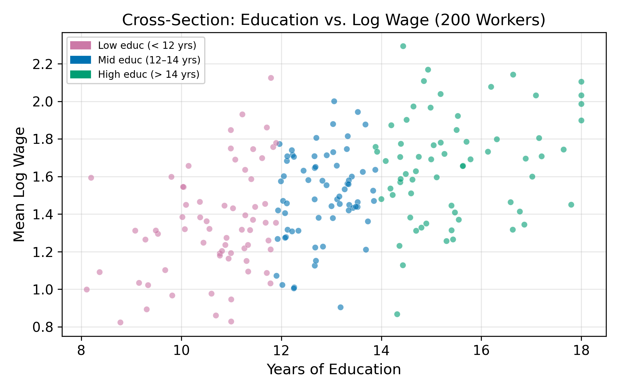
This is the classic ability bias problem from IV estimation, now in a panel setting. The difference: instead of searching for an external instrument like distance to college, we will exploit the panel structure itself.
We face a dilemma. The two standard panel estimators each fail in a different way.
13.2 FE Absorbs Education
The within transformation subtracts individual means from both sides of Equation 13.1:
\[ \log(\text{wage}_{it}) - \overline{\log(\text{wage})}_i = \beta_2(\text{exper}_{it} - \bar{\text{exper}}_i) + \beta_3(\text{union}_{it} - \bar{\text{union}}_i) + (\varepsilon_{it} - \bar{\varepsilon}_i) \tag{13.2}\]
Education and race are gone. Because \(\text{educ}_i = \bar{\text{educ}}_i\) for every period, the demeaned variable \(\text{educ}_i - \bar{\text{educ}}_i = 0\). The same applies to \(\text{black}_i\). Fixed effects eliminates the endogeneity problem by eliminating \(\alpha_i\), but it also eliminates everything that does not vary over time, including the coefficients we care about most.
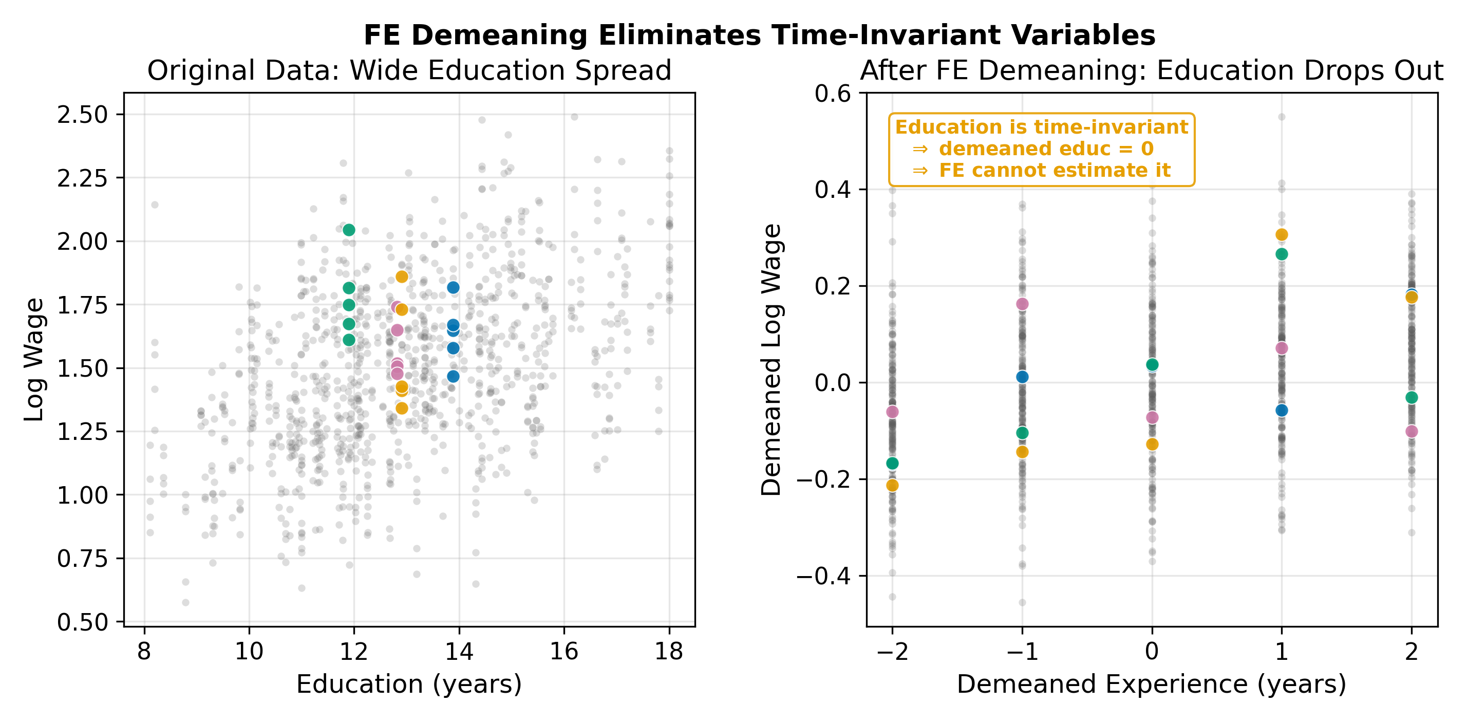
\(\implies\) FE gives consistent estimates of \(\beta_2\) and \(\beta_3\), but \(\beta_1\) and \(\beta_4\) are not identified.
13.3 RE Is Biased
Random effects can estimate \(\beta_1\) because it does not fully demean the data. It uses a partial demeaning controlled by \(\hat{\alpha}\), which preserves between-individual variation. But RE requires:
\[ \text{Cov}(\alpha_i, x_{kit}) = 0 \quad \text{for all regressors } x_k \tag{13.3}\]
If ability (\(\alpha_i\)) is correlated with education, this assumption fails. RE produces an estimate of \(\beta_1\), but that estimate is biased and inconsistent.
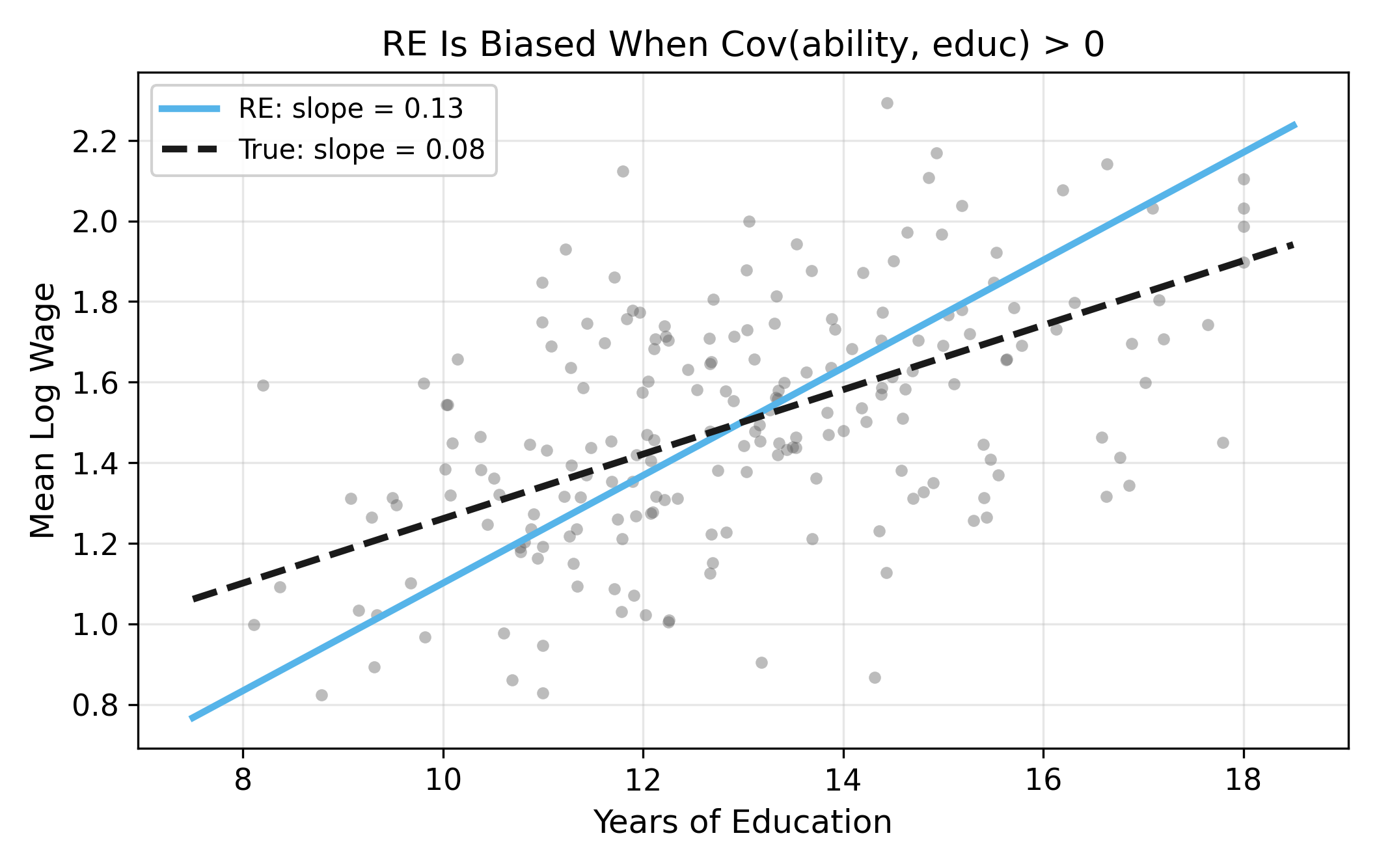
RE is biased whenever \(\alpha_i\) correlates with any regressor. The Hausman test (comparing FE and RE on the time-varying coefficients) detects exactly this situation.
The dilemma in full:
| Estimator | Estimates \(\beta_1\) (education)? | Consistent? |
|---|---|---|
| Fixed Effects | No | Yes (for time-varying coefficients) |
| Random Effects | Yes | No (if ability correlates with education) |
We need an estimator that can recover time-invariant coefficients while addressing the endogeneity of \(\alpha_i\). That is what Hausman and Taylor (1981) proposed.
13.4 The Hausman-Taylor Idea
The Hausman-Taylor estimator begins by classifying every variable in the model into one of four categories:
| Category | Notation | Time-varying? | Correlated with \(\alpha_i\)? | Example |
|---|---|---|---|---|
| Time-varying exogenous | \(X_1\) | Yes | No | Experience |
| Time-varying endogenous | \(X_2\) | Yes | Yes | Union membership |
| Time-invariant exogenous | \(Z_1\) | No | No | Race |
| Time-invariant endogenous | \(Z_2\) | No | Yes | Education |
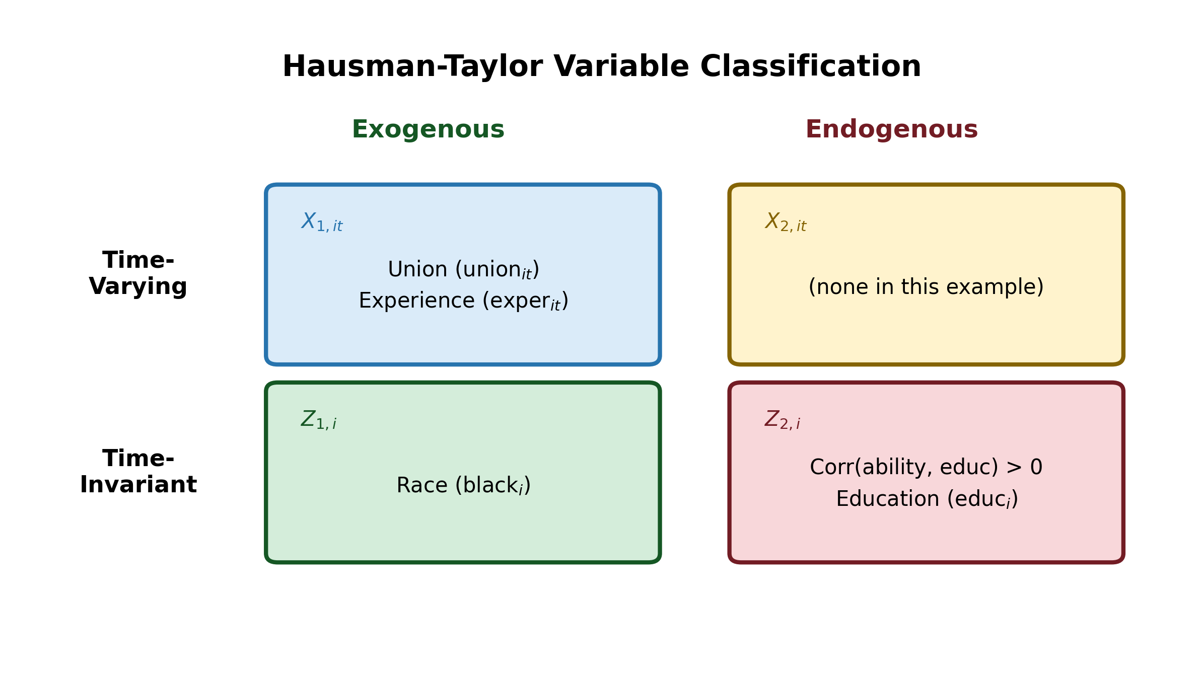
The word “endogenous” here means specifically correlated with \(\alpha_i\), not correlated with \(\varepsilon_{it}\). All variables are assumed uncorrelated with the idiosyncratic error.
13.4.1 The Instruments
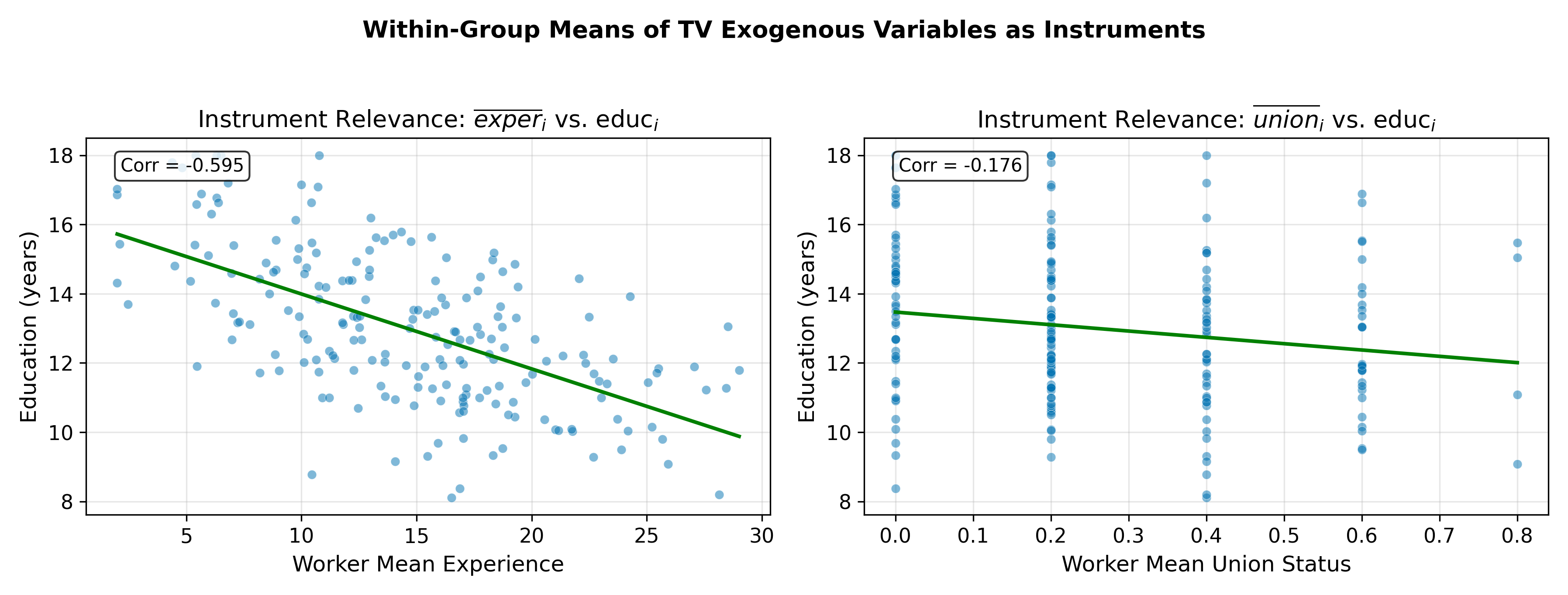
Here is the central insight. The within-group means of the time-varying exogenous variables, \(\bar{X}_{1,i}\), serve as instruments for the time-invariant endogenous variables \(Z_2\).
Why does this work? Consider experience as \(X_1\) and education as \(Z_2\). Individual average experience \(\bar{\text{exper}}_i\) varies across individuals and is correlated with education level (more educated workers may enter the labor force later, accumulating a different experience profile). But if experience is exogenous, meaning \(\text{Cov}(\text{exper}_{it}, \alpha_i) = 0\), then \(\bar{\text{exper}}_i\) is also uncorrelated with \(\alpha_i\). We have an instrument that is:
- Relevant: correlated with \(Z_2\) (education)
- Exogenous: uncorrelated with \(\alpha_i\) (the source of endogeneity)
No external data is required. The instruments come from the panel itself.
The insight: if experience is exogenous, then the individual’s average experience level across time periods provides variation that is correlated with education but uncorrelated with the individual effect.
The within-group mean \(\bar{X}_{1,i}\) is a between-individual quantity. It captures how person \(i\)’s typical level of a time-varying variable differs from other individuals. Because \(X_1\) is exogenous (uncorrelated with \(\alpha_i\)), its mean is also uncorrelated with \(\alpha_i\). But individual means of time-varying variables tend to correlate with time-invariant characteristics. For example, someone who enters the labor force at 18 (low education) has a different average experience path than someone who enters at 22 (college degree). This cross-individual variation in \(\bar{X}_{1,i}\) is what identifies \(\beta_{Z_2}\).
13.5 The HT Procedure
The estimator combines within estimation, IV estimation, and GLS in a three-step procedure.
Step 1: Within estimation. Run fixed effects on Equation 13.1. This produces consistent estimates \(\hat{\beta}_{X_1}\) and \(\hat{\beta}_{X_2}\) for the time-varying variables, along with residuals. The time-invariant coefficients are not estimated in this step.
Step 2: IV on the between equation. Construct individual-level residuals by averaging the original equation over time:
\[ \bar{y}_i = \beta_0 + \beta_{X_1} \bar{X}_{1,i} + \beta_{X_2} \bar{X}_{2,i} + \beta_{Z_1} Z_{1,i} + \beta_{Z_2} Z_{2,i} + \alpha_i + \bar{\varepsilon}_i \tag{13.4}\]
Using the consistent estimates from Step 1, define:
\[ d_i = \bar{y}_i - \hat{\beta}_{X_1} \bar{X}_{1,i} - \hat{\beta}_{X_2} \bar{X}_{2,i} = \beta_0 + \beta_{Z_1} Z_{1,i} + \beta_{Z_2} Z_{2,i} + \alpha_i + \bar{\varepsilon}_i + \text{estimation error} \tag{13.5}\]
Now run an IV regression of \(d_i\) on \(Z_1\) and \(Z_2\), using \(\bar{X}_{1,i}\) and \(Z_1\) as instruments. The instruments \(\bar{X}_{1,i}\) are uncorrelated with \(\alpha_i\) (by the exogeneity of \(X_1\)), and \(Z_1\) is uncorrelated with \(\alpha_i\) by assumption. This identifies \(\hat{\beta}_{Z_1}\) and \(\hat{\beta}_{Z_2}\).
Step 3: FGLS combination. Use the variance components estimated from Steps 1 and 2 to construct a GLS transformation. Apply this transformation to the full model and re-estimate all coefficients jointly. This final step combines within and between information efficiently, producing estimates that are more precise than either FE or the Step 2 IV estimates alone.
The order requirement: you need at least as many \(X_1\) variables as \(Z_2\) variables. If you have one time-invariant endogenous variable (education), you need at least one time-varying exogenous variable (experience) to serve as its instrument.
13.5.1 Instrument Count Requirement
For the IV regression in Step 2 to be identified, you need:
\[ \text{number of } X_1 \text{ variables} \geq \text{number of } Z_2 \text{ variables} \tag{13.6}\]
This is the standard order condition from IV estimation. If you have more \(X_1\) variables than \(Z_2\) variables, the model is overidentified, which allows for testing instrument validity.
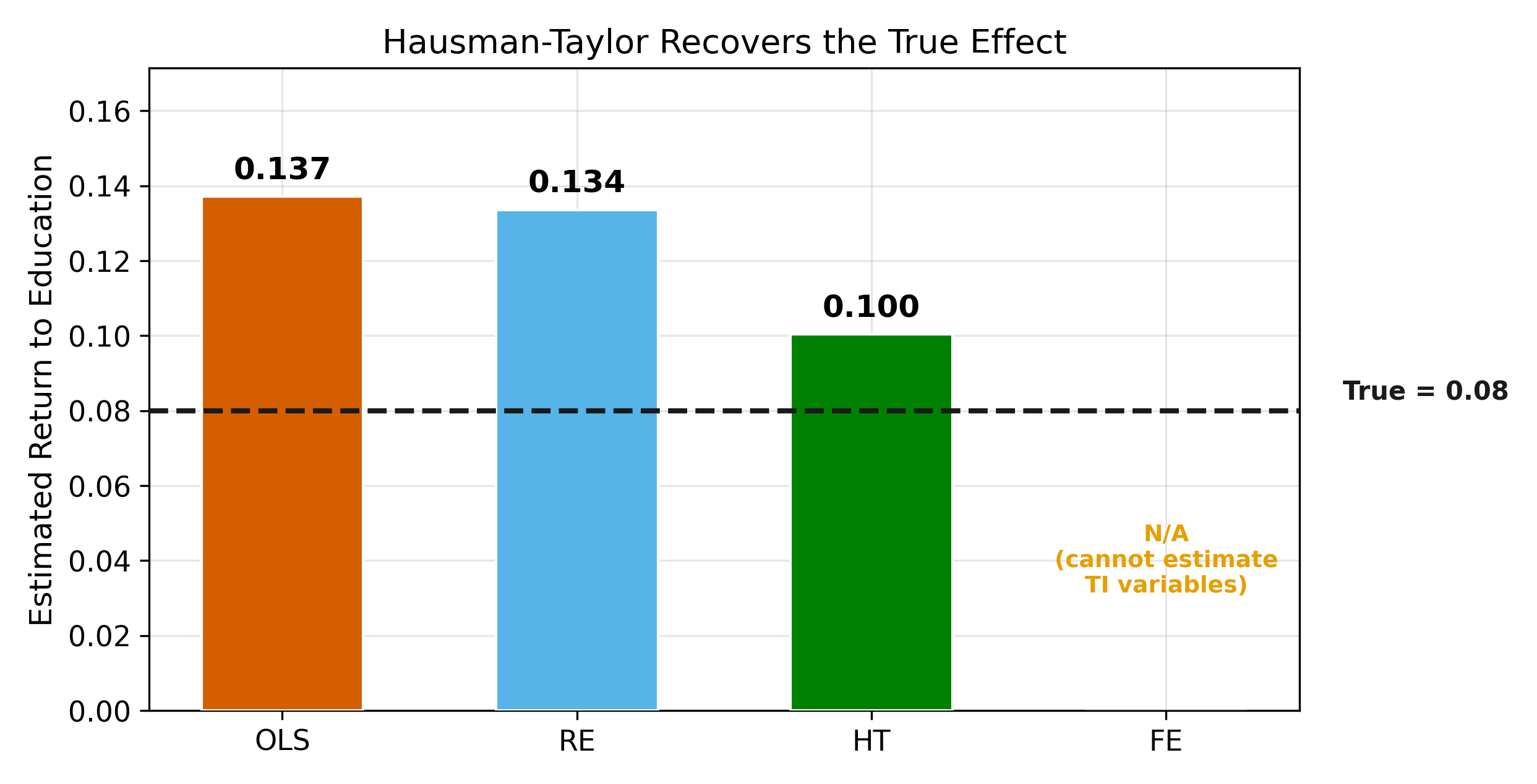
13.6 Results
How does the Hausman-Taylor estimator perform relative to FE and RE?
The comparison across all three estimators:
| FE | RE | HT | |
|---|---|---|---|
| Time-varying coefficients (\(\beta_{X_1}, \beta_{X_2}\)) | Consistent | Biased (if \(\text{Cov}(\alpha_i, X) \neq 0\)) | Consistent |
| Time-invariant exogenous (\(\beta_{Z_1}\)) | Not identified | Biased | Consistent |
| Time-invariant endogenous (\(\beta_{Z_2}\)) | Not identified | Biased | Consistent |
| Efficiency | Least efficient | Most efficient (if valid) | Between FE and RE |
\(\implies\) HT is the only estimator that produces consistent estimates of all four coefficient types.
When \(\text{Cov}(\alpha_i, X) = 0\) for all regressors, RE uses all available information optimally through GLS. HT imposes the same assumption on \(X_1\) and \(Z_1\) but treats \(X_2\) and \(Z_2\) as endogenous, using instruments rather than direct estimation. Instrumentation always costs precision: the IV estimates have larger standard errors than the corresponding GLS estimates. HT pays this efficiency cost to gain consistency when some variables are endogenous.
13.7 Testing HT Assumptions
The Hausman-Taylor estimator rests on assumptions that can be partially tested.
13.7.1 Overidentification Test
When the model is overidentified (more \(X_1\) variables than \(Z_2\) variables), a Sargan or Hansen test checks whether the instruments \(\bar{X}_{1,i}\) are jointly valid. The null hypothesis is that all instruments are uncorrelated with \(\alpha_i\). Rejection suggests that at least one \(X_1\) variable may not be truly exogenous.
13.7.2 Hausman Test: HT vs. FE
Compare the time-varying coefficients from HT to those from FE. Under correct specification of HT, both should be consistent for \(\beta_{X_1}\) and \(\beta_{X_2}\), and the estimates should be close.
\[ H = (\hat{\beta}_{TV}^{HT} - \hat{\beta}_{TV}^{FE})' [\widehat{\text{Var}}(\hat{\beta}_{TV}^{FE}) - \widehat{\text{Var}}(\hat{\beta}_{TV}^{HT})]^{-1} (\hat{\beta}_{TV}^{HT} - \hat{\beta}_{TV}^{FE}) \sim \chi^2_K \tag{13.7}\]
If this test rejects, the HT instruments may be invalid: a variable classified as \(X_1\) (time-varying exogenous) may actually belong in \(X_2\) (time-varying endogenous).
Rejection means the time-varying coefficients from HT and FE are statistically different. Since FE is always consistent for these coefficients (it does not rely on instrument validity), the problem must be with HT. Specifically, the instruments \(\bar{X}_{1,i}\) are not truly exogenous, meaning that some variable you classified as time-varying exogenous is actually correlated with \(\alpha_i\). You need to reclassify that variable as \(X_2\) and find a different instrument, or accept that HT is not appropriate for your data.
The Hausman test (HT vs FE) tests the instrument validity assumption. The overidentification test serves a similar purpose but focuses specifically on surplus instruments.
13.8 When HT Works (and When It Doesn’t)
The Hausman-Taylor estimator is not a universal solution. Its usefulness depends on the structure of your data.
HT works well when:
- You have enough time-varying exogenous variables to instrument for the time-invariant endogenous ones (the order condition in Equation 13.6 is satisfied)
- The within-group means \(\bar{X}_{1,i}\) are strongly correlated with \(Z_2\) (the instruments are relevant, not weak)
- The classification of variables into the four categories is defensible on economic grounds
HT fails when:
- All time-varying variables are endogenous (no \(X_1\) variables \(\implies\) no internal instruments)
- The within-group means \(\bar{X}_{1,i}\) are only weakly correlated with \(Z_2\) (weak instruments produce unreliable estimates, just as in standard IV)
- The researcher cannot credibly distinguish exogenous from endogenous variables (misclassification invalidates the entire procedure)
\(\implies\) The estimator is only as good as the variable classification. If you cannot defend why a particular time-varying variable is uncorrelated with \(\alpha_i\), the HT estimates are no more trustworthy than RE.
13.8.1 Comparison with External IV
An alternative to HT is to find an external instrument for \(Z_2\) and run a standard IV regression. For example, using distance to the nearest college as an instrument for education (as in Card, 1995). External IV does not require panel data at all, but good instruments are hard to find and must be argued on a case-by-case basis. HT avoids this by generating instruments internally from the panel structure. The tradeoff: external instruments can be stronger and more transparent, but HT is available whenever the panel contains time-varying exogenous variables.
When you have a credible, strong external instrument. External IV is conceptually simpler and does not require classifying every variable in the model. It also does not assume that any time-varying variable is uncorrelated with \(\alpha_i\). If you are uncertain about the exogeneity of your time-varying variables, external IV sidesteps that problem entirely. HT is most useful when no credible external instrument exists but the panel structure provides plausible internal instruments.
Return to the Panel Data Models hub for the full set of panel data topics, including the discussion problems where HT is applied (Problem 15.21(e)).