18 Count Data Models
Poisson, Negative Binomial, and Overdispersion
Count outcomes (number of doctor visits, patents filed, accidents per intersection) violate OLS assumptions: they are non-negative, integer-valued, and often right-skewed. Poisson regression uses a log link to model the conditional mean, but assumes equidispersion. When variance exceeds the mean, the negative binomial model adds a dispersion parameter.
This page is part of the Qualitative and Limited Dependent Variable Models chapter. You should be comfortable with maximum likelihood estimation and the idea that different dependent variable structures require different models. The binary choice background in Binary Choice Models is helpful but not strictly required.
18.1 OLS on Count Data
Suppose we want to model the number of doctor visits per year as a function of age, insurance status, and a self-reported health index. The dependent variable \(y_i\) takes values \(0, 1, 2, 3, \ldots\) with no upper bound but a strong concentration near zero and a long right tail. In a typical sample, most people report 0-3 visits, a smaller group reports 5-10, and a few outliers report 20 or more.
Running OLS on this outcome produces:
\[ \text{Visits}_i = \beta_0 + \beta_1 \text{Age}_i + \beta_2 \text{Insurance}_i + \beta_3 \text{Health}_i + \varepsilon_i \tag{18.1}\]
Three problems emerge immediately:
- Negative predictions. OLS can predict \(\hat{y} = -1.7\) for a young, healthy person without insurance. Negative doctor visits are impossible.
- Non-integer predictions. A predicted value of 3.4 visits has no natural interpretation for a count outcome.
- Constant marginal effects. OLS forces each additional year of age to add the same number of predicted visits, regardless of whether the person currently averages 0.5 or 15 visits per year. For count data, effects should be multiplicative, not additive.
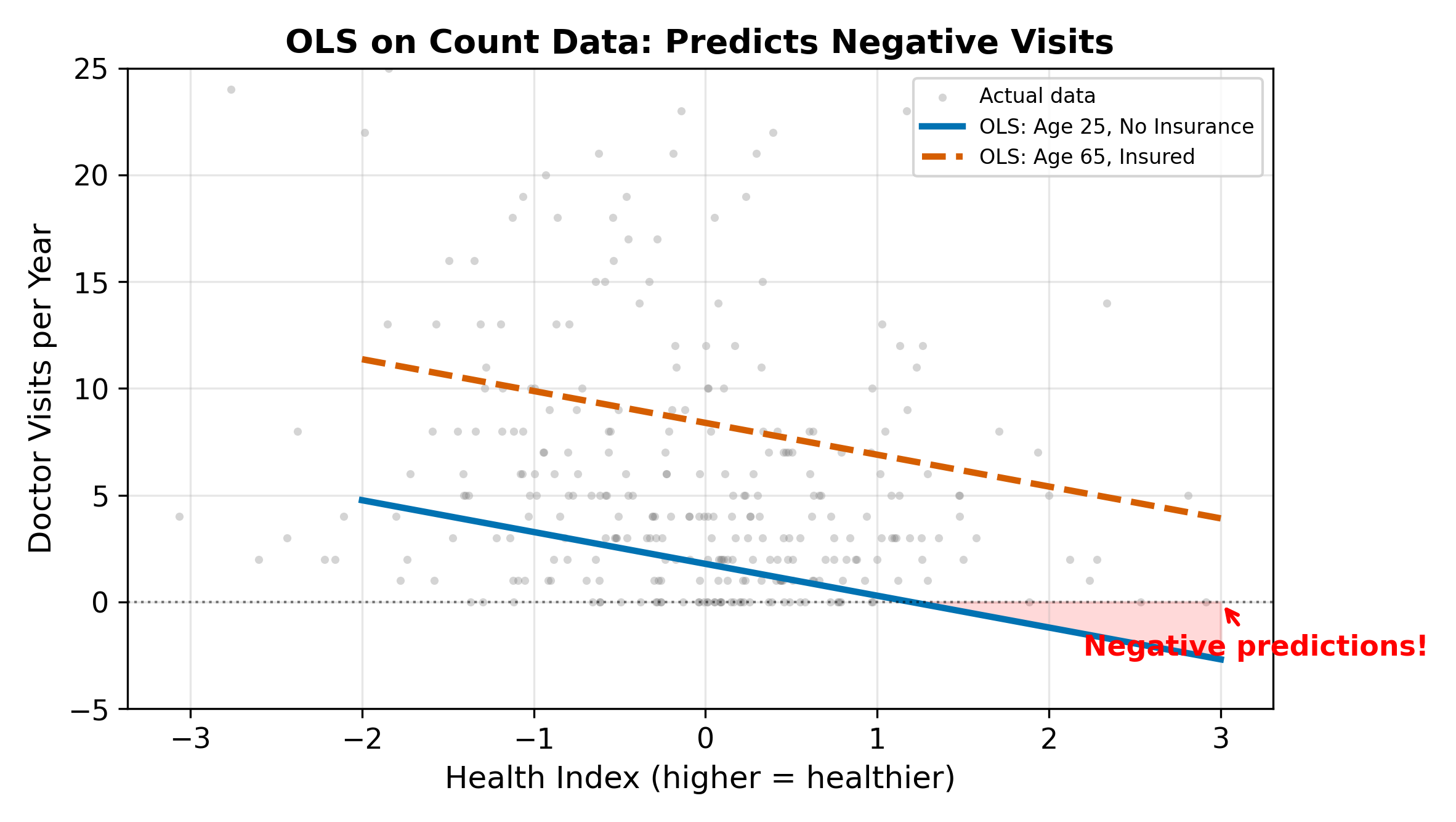
With enough data and a large mean, OLS gets the average marginal effect approximately right. But the model is misspecified: it ignores the non-negativity constraint and the discrete, skewed nature of the outcome.
\(\implies\) We need a model that respects the non-negative, integer-valued structure of count data and produces multiplicative rather than additive effects.
18.2 The Poisson Model
18.2.1 The Poisson Distribution
The Poisson distribution describes the probability of observing exactly \(k\) events in a fixed interval:
\[ P(Y = k) = \frac{e^{-\mu} \mu^k}{k!}, \qquad k = 0, 1, 2, \ldots \tag{18.2}\]
The single parameter \(\mu > 0\) controls both the mean and the variance:
\[ E[Y] = \mu, \qquad \text{Var}(Y) = \mu \tag{18.3}\]
This equality of mean and variance is called equidispersion. It will become the central issue of this page.
18.2.2 The Log Link
To connect the Poisson mean to covariates, we use a log link:
\[ \ln(\mu_i) = \beta_0 + \beta_1 \text{Age}_i + \beta_2 \text{Insurance}_i + \beta_3 \text{Health}_i \tag{18.4}\]
Equivalently, exponentiating both sides:
\[ \mu_i = e^{\beta_0 + \beta_1 \text{Age}_i + \beta_2 \text{Insurance}_i + \beta_3 \text{Health}_i} \tag{18.5}\]
The exponential function guarantees \(\mu_i > 0\) for any values of the covariates and any coefficient values. This solves the negative-prediction problem that plagues OLS.
The log link is not a transformation of the dependent variable. We do not take \(\ln(y_i)\) (which is undefined when \(y_i = 0\)). Instead, the log link operates on the conditional mean \(\mu_i\).
18.2.3 Maximum Likelihood Estimation
The log-likelihood for the Poisson regression model is:
\[ \ell(\beta) = \sum_{i=1}^{N} \left[ y_i \ln \mu_i - \mu_i - \ln(y_i!) \right] \tag{18.6}\]
where \(\mu_i = e^{X_i \beta}\). Substituting:
\[ \ell(\beta) = \sum_{i=1}^{N} \left[ y_i (X_i \beta) - e^{X_i \beta} - \ln(y_i!) \right] \tag{18.7}\]
The last term does not depend on \(\beta\) and drops out of the optimization. MLE finds the \(\hat{\beta}\) that maximizes this expression. The resulting estimator is consistent and asymptotically normal under standard regularity conditions.
18.2.4 Interpreting Poisson Coefficients
The coefficients have a semi-elasticity interpretation. Since \(\ln(\mu_i) = X_i \beta\), a one-unit increase in \(x_k\) changes \(\ln(\mu)\) by \(\beta_k\). In percentage terms:
\[ \frac{\Delta \mu}{\mu} \approx \beta_k \quad \text{(for small } \beta_k \text{)} \tag{18.8}\]
More precisely, increasing \(x_k\) by one unit multiplies the expected count by \(e^{\beta_k}\). For a dummy variable going from 0 to 1, the exact percentage change in the mean is \((e^{\beta_k} - 1) \times 100\%\).
This multiplicative structure is natural for count data. A treatment that doubles doctor visits for someone averaging 2 visits (from 2 to 4) also doubles visits for someone averaging 10 (from 10 to 20). The absolute increase differs, but the proportional effect is constant. OLS, by contrast, forces the same absolute increase regardless of the baseline.
The expected count is multiplied by \(e^{0.3} = 1.35\). So predicted visits increase by 35%. If a person without insurance was predicted to have 4 visits, the same person with insurance is predicted to have \(4 \times 1.35 = 5.4\) visits.
The semi-elasticity approximation (\(\approx 30\%\)) is close but understates the exact effect. The approximation works best when \(|\beta_k|\) is small (say, below 0.1).
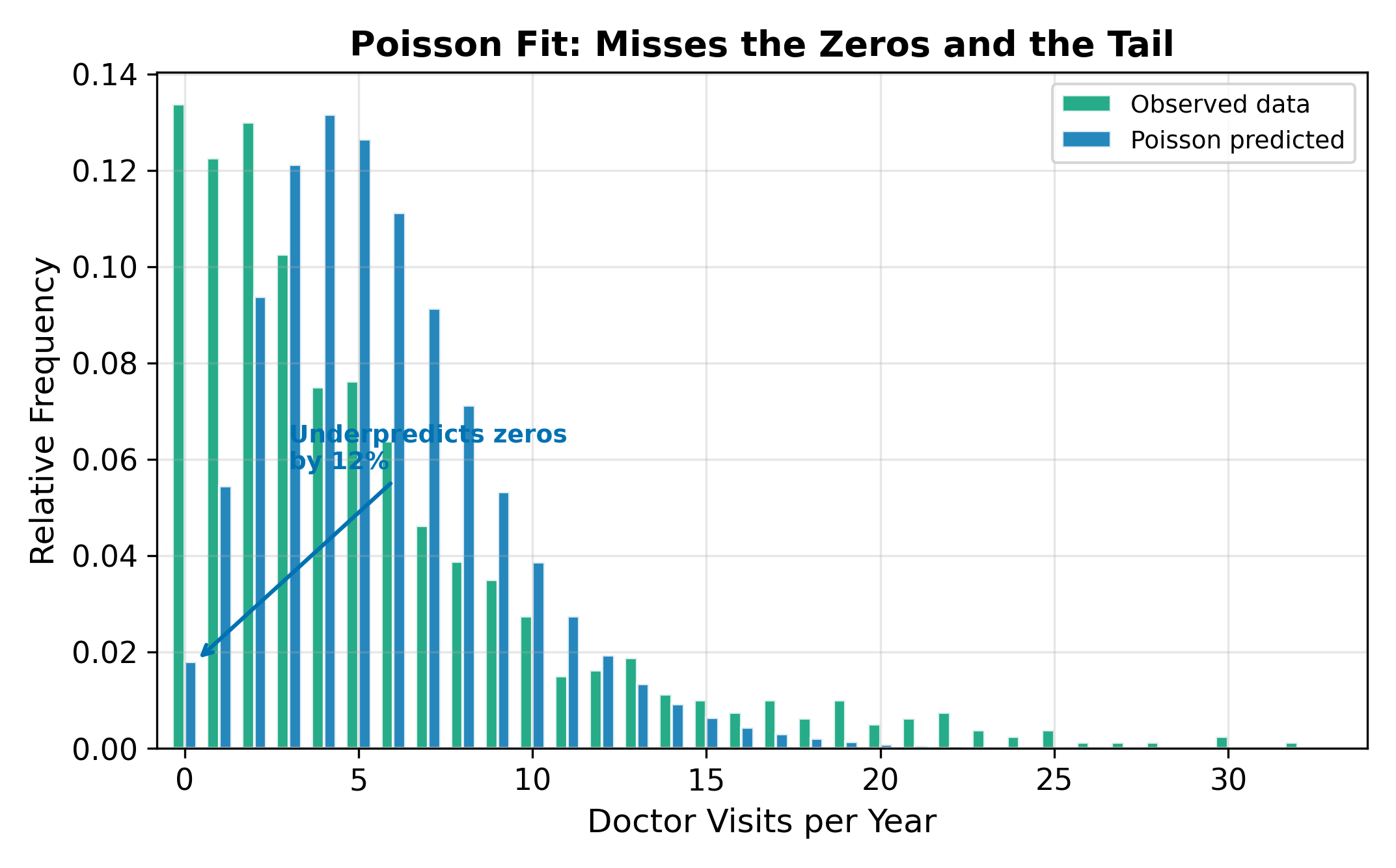
18.3 The Equidispersion Problem
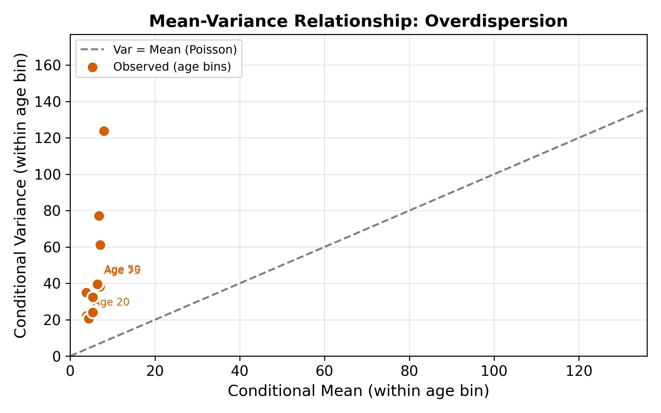
The Poisson model’s defining restriction is equidispersion: \(E[Y] = \text{Var}(Y) = \mu\). This is an extremely strong assumption. In practice, real count data almost always exhibit overdispersion, where the variance exceeds the mean:
\[ \text{Var}(Y) > E[Y] \]
Why does overdispersion arise? The usual culprit is unobserved heterogeneity. Even after controlling for age, insurance, and health status, some people visit the doctor more than others for reasons we cannot measure (anxiety, proximity to a clinic, family history). This latent variation inflates the variance beyond what the Poisson model allows.
18.3.1 A Quick Diagnostic
A simple first check: compute the sample mean \(\bar{y}\) and sample variance \(s^2\) of the dependent variable. If \(s^2 / \bar{y}\) is substantially greater than 1, overdispersion is likely present. In the doctor visits data, a ratio of 3 or 4 is common. More formal tests (Cameron-Trivedi, Dean-Lawless) are available, but the variance-to-mean ratio gives immediate intuition.
18.3.2 Consequences of Ignoring Overdispersion
When overdispersion is present but we estimate Poisson anyway:
- Point estimates remain consistent. The Poisson quasi-MLE is consistent for \(\beta\) as long as the conditional mean \(E[Y|X] = e^{X\beta}\) is correctly specified, even if the variance assumption is wrong.
- Standard errors are too small. The Poisson model assumes \(\text{Var}(Y|X) = \mu\), but the true variance is larger. This means the estimated information matrix overstates precision.
- Tests reject too often. Artificially small standard errors lead to inflated \(t\)-statistics. Variables appear statistically significant when they are not.
Overdispersion does not bias Poisson point estimates. It only corrupts the standard errors. This is analogous to heteroskedasticity in OLS: the coefficients are still unbiased, but inference based on the usual standard errors is unreliable.
\(\implies\) Even if the Poisson coefficients are roughly correct, you cannot trust hypothesis tests from a Poisson model when overdispersion is present. You need either robust standard errors or a different model.
18.4 Negative Binomial Regression
18.4.1 Relaxing Equidispersion
The negative binomial (NB) model generalizes Poisson by allowing the variance to exceed the mean. The conditional variance takes the form:
\[ \text{Var}(Y_i | X_i) = \mu_i + \alpha \mu_i^2 \tag{18.9}\]
where \(\alpha \geq 0\) is the overdispersion parameter. The conditional mean is the same as in Poisson:
\[ E[Y_i | X_i] = \mu_i = e^{X_i \beta} \tag{18.10}\]
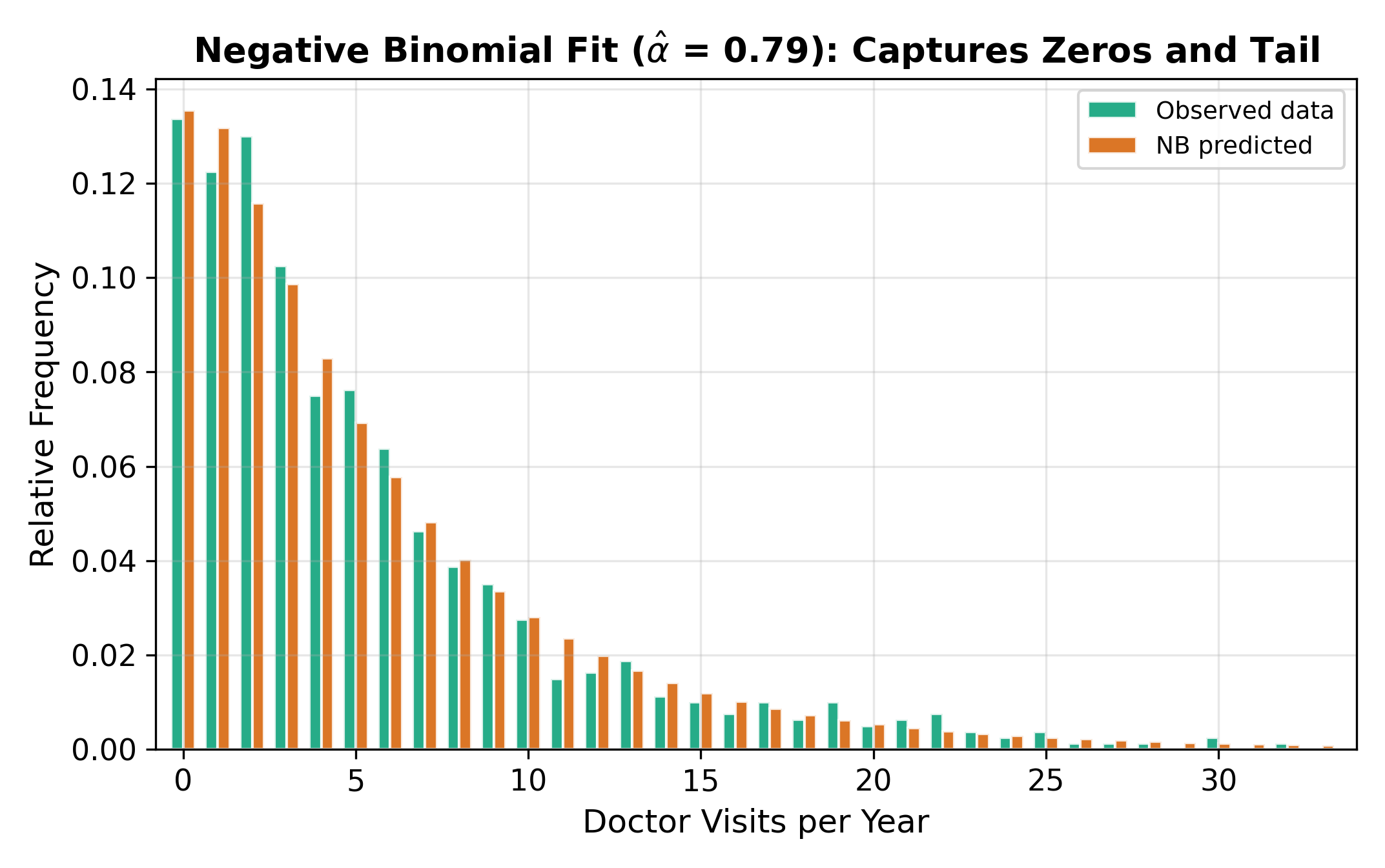
When \(\alpha = 0\), the variance equals the mean and the NB model reduces to Poisson. When \(\alpha > 0\), the variance is strictly larger than the mean, accommodating overdispersion.
18.4.2 Where the NB Distribution Comes From
The negative binomial arises from a natural generalization of the Poisson. Suppose the Poisson rate parameter \(\mu_i\) is not fixed but varies across individuals according to a Gamma distribution, reflecting unobserved heterogeneity. Integrating out this Gamma heterogeneity produces the negative binomial distribution. The parameter \(\alpha\) captures how much unobserved variation exists beyond what the covariates explain.
18.4.3 Testing for Overdispersion
The hypothesis \(H_0: \alpha = 0\) tests whether the Poisson restriction holds. If rejected, the data exhibit overdispersion and the NB model is preferred. Most software reports this test automatically when estimating a negative binomial model.
Poisson. If the data are consistent with equidispersion, the Poisson model is more parsimonious (one fewer parameter) and its standard errors are valid. The NB model would still produce consistent estimates, but the extra parameter adds noise without improving the model. This parallels the logic of using homoskedastic standard errors when a Breusch-Pagan test fails to reject.
18.4.4 Poisson vs. Negative Binomial: Visual Comparison
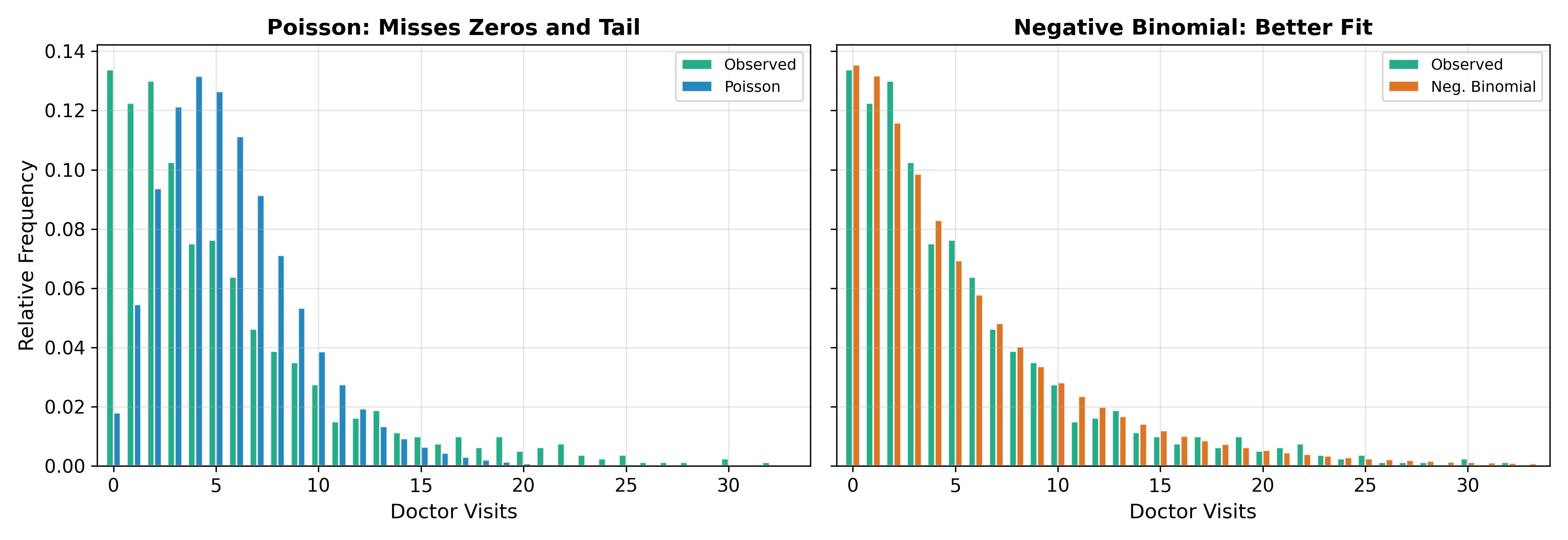
The figure above illustrates the practical difference. The Poisson distribution is too narrow: it underpredicts zeros and underpredicts large counts. The negative binomial, with its extra dispersion parameter, accommodates both the excess zeros and the heavy right tail that are typical of real count data.
18.4.5 NB Coefficient Interpretation
Because the conditional mean has the same log-link form as Poisson (\(\mu_i = e^{X_i \beta}\)), the NB coefficients carry the same semi-elasticity interpretation. A one-unit increase in \(x_k\) multiplies the expected count by \(e^{\beta_k}\). The only difference is in the standard errors and the model’s treatment of dispersion. In practice, NB and Poisson point estimates are often numerically close, with the NB intervals being wider.
18.5 Coefficient Comparison
How different are the coefficient estimates across the three approaches? In most applications, the point estimates from OLS, Poisson, and NB are similar in sign and approximate magnitude. The differences show up in the standard errors.
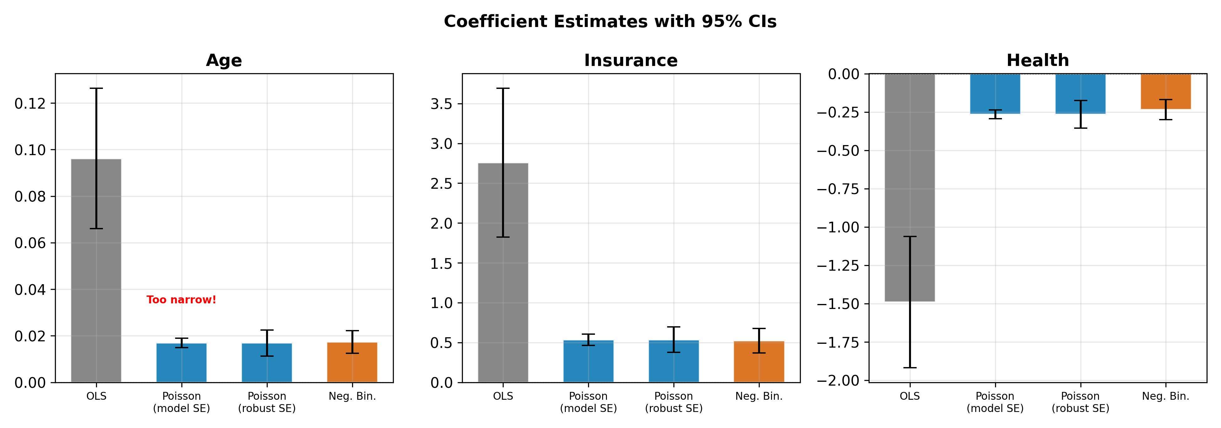
The pattern in Figure 18.6 is typical:
- OLS, Poisson, and NB agree on the direction and rough size of each effect.
- Poisson standard errors are the smallest because the model assumes the tightest variance structure.
- NB standard errors are larger, reflecting the additional uncertainty from overdispersion.
- OLS standard errors fall somewhere in between, but OLS predictions violate the non-negativity constraint.
Quasi-Poisson is a quick fix: it adjusts Poisson standard errors by \(\sqrt{\hat{\phi}}\), where \(\hat{\phi}\) is the estimated dispersion parameter, without specifying the full NB distribution. This corrects inference without changing the point estimates.
\(\implies\) If you only care about the direction of effects, Poisson and NB give similar answers. If you care about statistical significance (and you should), the choice between Poisson and NB can flip a conclusion from “significant” to “not significant.”
18.6 Excess Zeros
Sometimes the data contain more zeros than either Poisson or NB can accommodate. A person might report zero doctor visits for two distinct reasons: they are healthy and have no need (a “structural zero”), or they face barriers to access and would visit if they could (a “sampling zero”). A single Poisson or NB model conflates both sources of zeros.
Zero-inflated models address this by combining two processes:
- A binary model (logit or probit) determines whether the observation is a structural zero.
- A count model (Poisson or NB) generates the count for observations that pass the first stage.
The resulting predicted probability of zero is a mixture:
\[ P(Y_i = 0) = \pi_i + (1 - \pi_i) \cdot P_{\text{count}}(Y_i = 0) \tag{18.11}\]
where \(\pi_i\) is the probability of being a structural zero. When \(\pi_i = 0\) for all observations, the model reduces to standard Poisson or NB.
The Vuong test compares a standard count model to its zero-inflated counterpart. A significant test statistic favors the zero-inflated version.
Zero-inflated Poisson (ZIP) and zero-inflated negative binomial (ZINB) are available in most statistical software. The full treatment of these models is beyond the scope of this page, but the logic is straightforward: if the zero-generating process differs from the count-generating process, model them separately.
A related model is the hurdle model, which also separates zeros from positives but uses a different structure: a binary model governs whether \(y = 0\) or \(y > 0\), and a truncated count model governs the positive counts. The distinction is subtle: zero-inflated models allow zeros to come from both processes, while hurdle models assign all zeros to the binary stage.
Tobit and Censored Regression covers the case where the dependent variable is continuous but censored at a boundary (e.g., hours worked piling up at zero). See also the hub page for the full limited dependent variable roadmap.