20 The Heckman Selection Model
Correcting for Sample Selection Bias with the Inverse Mills Ratio
We observe wages only for workers. If the decision to work is correlated with unobserved determinants of wages (e.g., motivation), OLS on workers only is biased. Heckman’s two-step procedure models the selection process with a probit, constructs the inverse Mills ratio as a sufficient statistic for selection bias, and includes it as an additional regressor in the wage equation.
This page is part of the Qualitative and Limited Dependent Variable Models sequence. You should be comfortable with:
- Binary choice models (probit estimation, latent variable framework)
- The Tobit model (censored data, the distinction between participation and amount)
- Instrumental variables (endogeneity, exclusion restrictions)
20.1 The Problem: Missing Wages
Consider a standard wage equation:
\[ \log(\text{wage}_i) = \beta_0 + \beta_1 \, \text{educ}_i + \beta_2 \, \text{exper}_i + u_i \tag{20.1}\]
We want to estimate the return to education (\(\beta_1\)) and the return to experience (\(\beta_2\)). But we only observe wages for people who work. Non-workers have no wage data. Their \(y\) is missing.
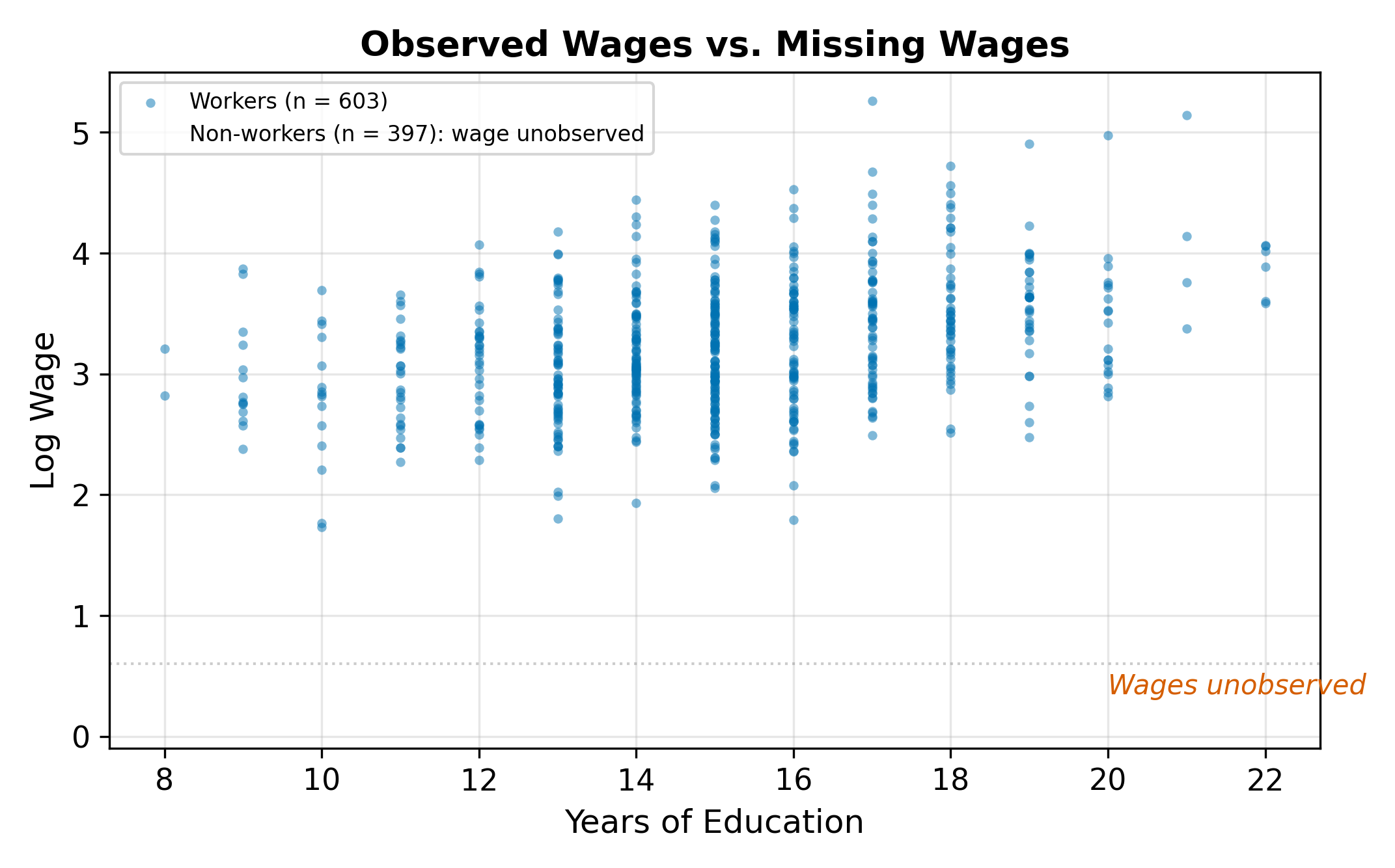
If the missing observations were randomly scattered, we could just run OLS on the workers and lose some precision but avoid bias. The problem is that the missingness is not random. People who choose to work are a self-selected group. They may have higher motivation, better labor market opportunities, or fewer outside options than non-workers.
This is not the same as missing data at random. The missingness depends on the outcome itself: people with higher potential wages are more likely to work, so the observed sample overrepresents high earners.
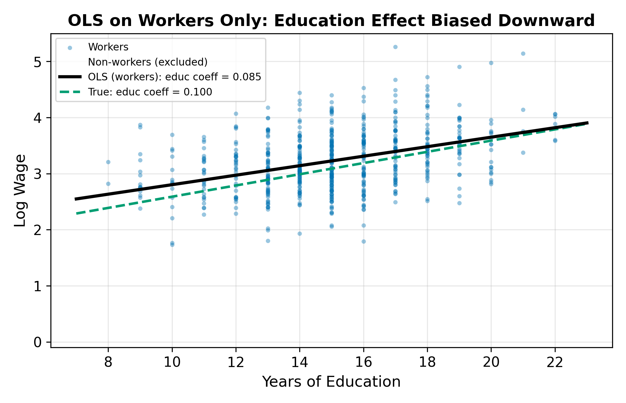
Think of it this way. Suppose you wanted to estimate the average height of all Americans, but your sample consists entirely of NBA players. You would massively overestimate the population mean because your sample is selected on an outcome (basketball ability) that correlates with the variable you are trying to measure (height). OLS on workers only makes the same mistake: it estimates a wage equation from a sample selected on a variable (the decision to work) that correlates with wages themselves.
This problem is pervasive in economics. We observe wages only for workers, medical expenditures only for patients who seek care, loan performance only for borrowers who were approved, and auction prices only for items that sold. In each case, running OLS on the observed sample ignores the process that determined which observations we see.
\(\implies\) OLS on the selected sample does not recover the population parameters. We need a method that accounts for how the sample was selected.
20.2 The Selection Problem
The full model has two equations and two error terms.
Selection equation (determines who works):
\[ \text{work}_i^* = \gamma_0 + \gamma_1 \, \text{educ}_i + \gamma_2 \, \text{kids}_i + \gamma_3 \, \text{spouse\_inc}_i + v_i \tag{20.2}\]
Person \(i\) works if \(\text{work}_i^* > 0\). We observe wages only when \(\text{work}_i^* > 0\).
Outcome equation (determines wages for workers):
\[ \log(\text{wage}_i) = \beta_0 + \beta_1 \, \text{educ}_i + \beta_2 \, \text{exper}_i + u_i \tag{20.3}\]
The errors \(u_i\) and \(v_i\) are assumed jointly normal:
\[ \begin{pmatrix} u_i \\ v_i \end{pmatrix} \sim N\left(\begin{pmatrix} 0 \\ 0 \end{pmatrix}, \begin{pmatrix} \sigma_u^2 & \rho\sigma_u \\ \rho\sigma_u & 1 \end{pmatrix}\right) \tag{20.4}\]
The variance of \(v_i\) is normalized to 1 (as in any probit). The parameter \(\rho\) is the correlation between the two errors. If \(\rho \neq 0\), the unobserved factors driving the work decision are correlated with the unobserved factors driving wages. This is the source of the selection bias.
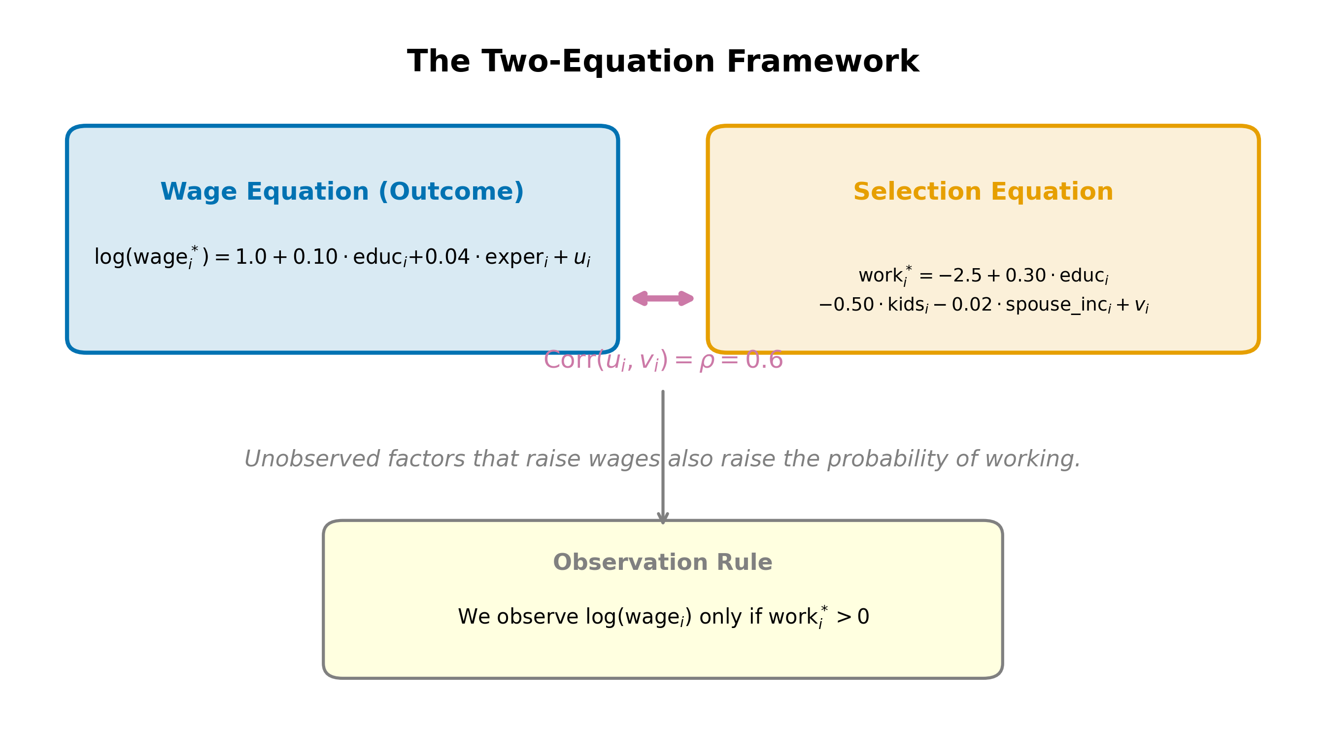
When \(\rho > 0\), people with positive wage shocks (\(u > 0\)) are also more likely to have positive selection shocks (\(v > 0\)), making them more likely to work. The observed sample overrepresents individuals with high unobserved wage determinants. When \(\rho < 0\), the reverse holds.
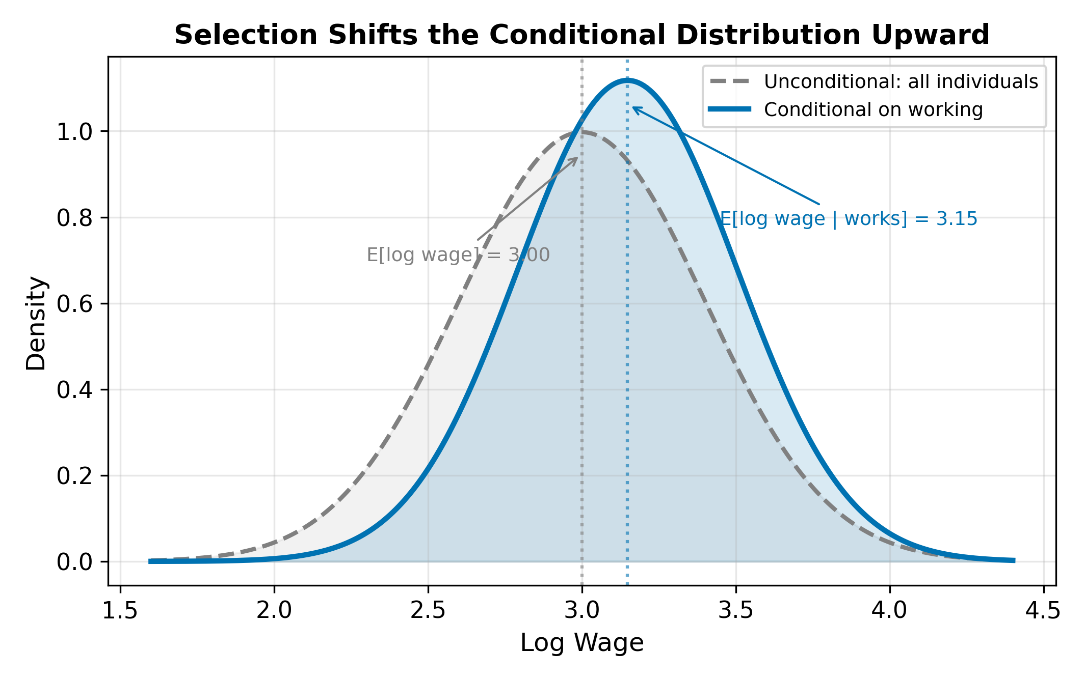
To see how this biases OLS, write the conditional expectation of wages among workers:
\[ E[\log(\text{wage}_i) \mid \text{works}] = \beta_0 + \beta_1 \, \text{educ}_i + \beta_2 \, \text{exper}_i + E[u_i \mid v_i > -\gamma' Z_i] \tag{20.5}\]
The last term is not zero. It depends on the selection variables \(Z_i\), and since some of those variables (like education) also appear in the wage equation, the omitted term correlates with the regressors. This is a classic omitted variable bias problem, where the omitted variable is a nonlinear function of the selection characteristics.
Positive. Motivation increases both \(u\) (wage residual) and \(v\) (selection residual), so \(\rho > 0\). The observed sample of workers contains disproportionately motivated people, inflating the average residual. The conditional expectation \(E[u_i \mid \text{works}] > 0\), which biases the intercept upward and can bias slope coefficients as well if motivation correlates with the regressors (e.g., motivated people also acquire more education).
20.3 The Inverse Mills Ratio
The conditional expectation of the wage error among workers is:
\[ E[u_i \mid \text{work}_i^* > 0] = \rho \, \sigma_u \cdot \lambda_i \tag{20.6}\]
where \(\lambda_i\) is the inverse Mills ratio, defined as:
\[ \lambda_i = \frac{\phi(\gamma' Z_i)}{\Phi(\gamma' Z_i)} \tag{20.7}\]
Here \(\gamma' Z_i = \gamma_0 + \gamma_1 \, \text{educ}_i + \gamma_2 \, \text{kids}_i + \gamma_3 \, \text{spouse\_inc}_i\) is the selection index, \(\phi\) is the standard normal PDF, and \(\Phi\) is the standard normal CDF.
The name “Mills ratio” comes from statistician John P. Mills, who studied the ratio \(\Phi(z)/\phi(z)\) in 1926. The inverse Mills ratio flips this to \(\phi(z)/\Phi(z)\). In the Heckman context, the argument \(z = \gamma' Z_i\) is evaluated at the selection index.
The inverse Mills ratio captures how much information the selection decision provides about the wage error. Consider two people:
- Person A has characteristics that make working almost certain (\(\gamma' Z\) large, \(\Phi(\gamma' Z) \approx 1\)). The fact that A works tells us almost nothing about their unobserved wage determinants. Their \(\lambda\) is small.
- Person B has characteristics that make working unlikely (\(\gamma' Z\) small, \(\Phi(\gamma' Z)\) small). The fact that B works despite the odds is informative: B probably has unusually favorable unobserved characteristics. Their \(\lambda\) is large.
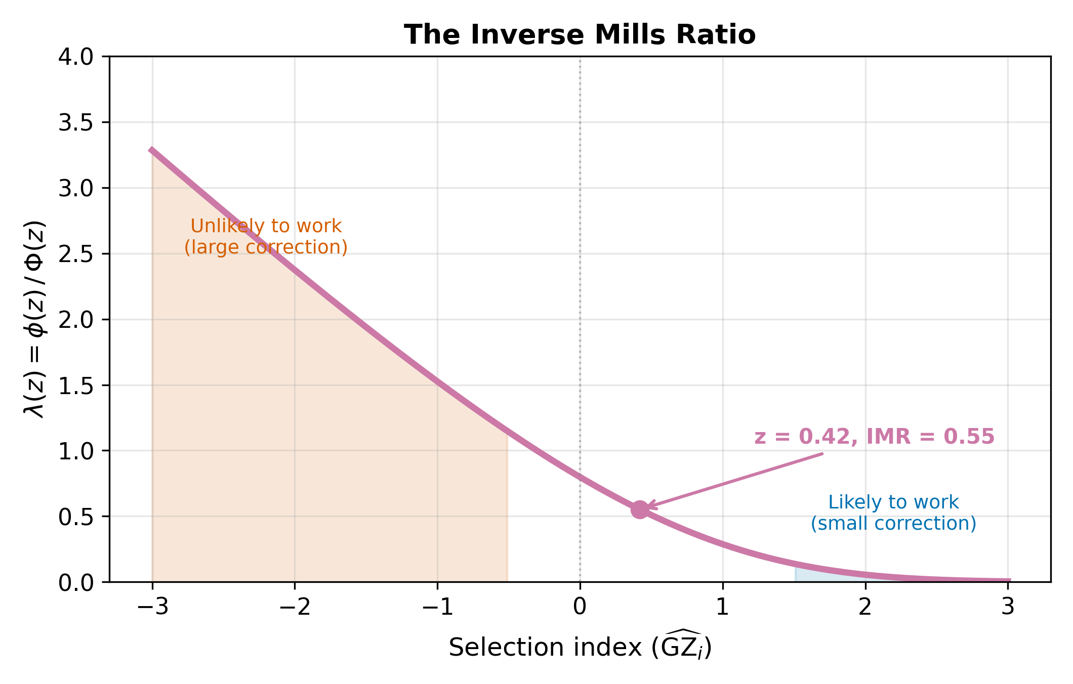
\(\lambda\) is always positive and decreasing in \(\gamma' Z\). Someone very likely to work (\(\gamma' Z\) large) has a small \(\lambda\): their selection provides little information about their unobserved wage determinants.
\(\implies\) The inverse Mills ratio is a sufficient statistic for the selection bias. If we include it in the wage equation, it absorbs the bias, leaving the remaining error uncorrelated with the regressors.
20.4 The Two-Step Procedure
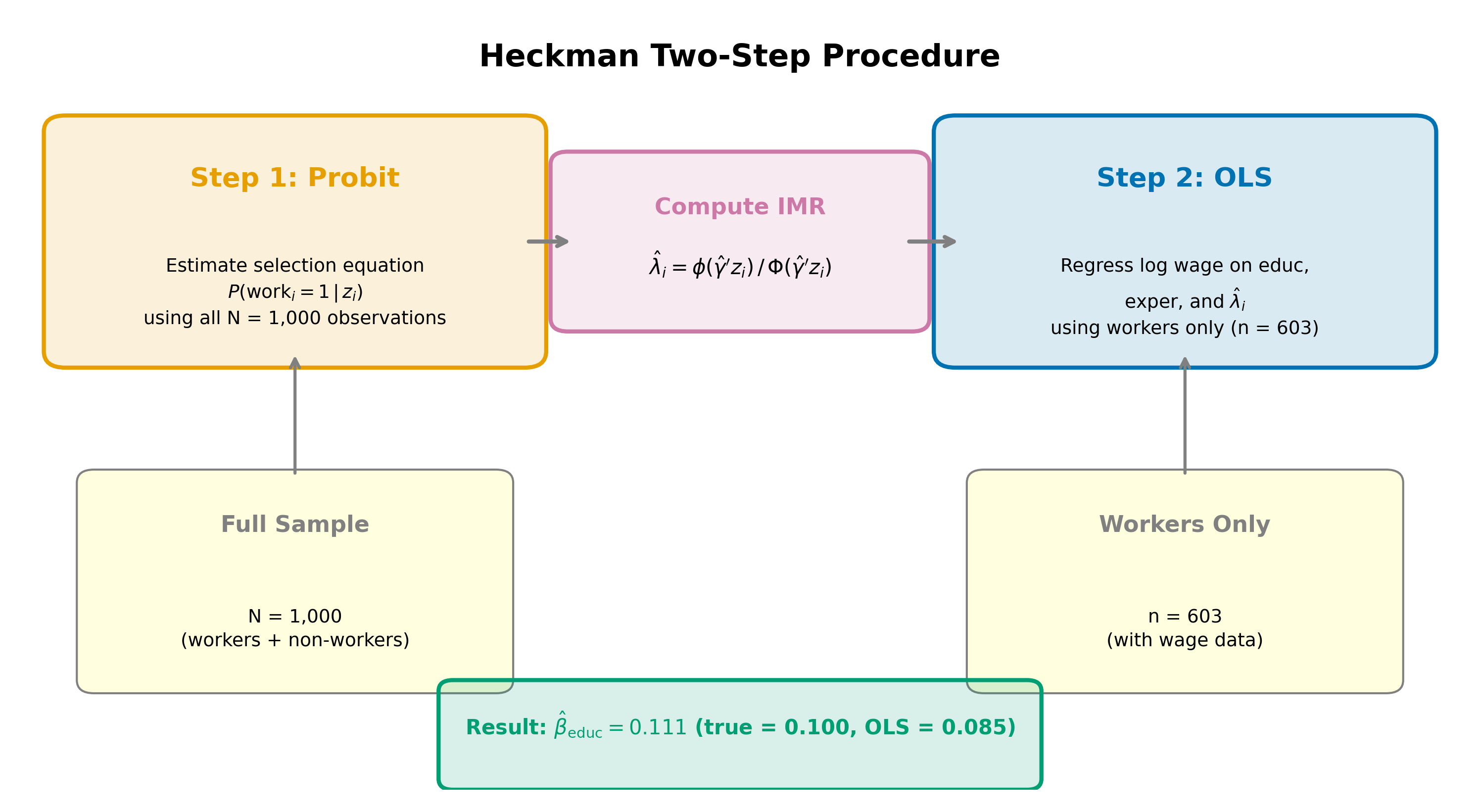
Heckman’s two-step estimator (also called Heckit) proceeds as follows.
Step 1: Estimate the selection equation. Run a probit of the work indicator on the selection variables (\(\text{educ}\), \(\text{kids}\), \(\text{spouse\_inc}\)). Use the estimated coefficients \(\hat{\gamma}\) to compute the fitted inverse Mills ratio for each worker:
\[ \hat{\lambda}_i = \frac{\phi(\hat{\gamma}' Z_i)}{\Phi(\hat{\gamma}' Z_i)} \tag{20.8}\]
Step 2: Include \(\hat{\lambda}\) in the outcome equation. Run OLS on workers only, adding \(\hat{\lambda}_i\) as an additional regressor:
\[ \log(\text{wage}_i) = \beta_0 + \beta_1 \, \text{educ}_i + \beta_2 \, \text{exper}_i + \delta \, \hat{\lambda}_i + \text{error}_i \tag{20.9}\]
The coefficient on the inverse Mills ratio is \(\delta = \rho \, \sigma_u\), the product of the error correlation and the standard deviation of the wage error.
The standard errors from Step 2 OLS are incorrect because \(\hat{\lambda}\) is an estimated regressor, not observed data. Murphy-Topel (or bootstrap) corrections are needed. Most software implements maximum likelihood estimation of both equations simultaneously, which avoids this issue.
Why does this work? From Equation 20.6, the expected wage among workers is:
\[ E[\log(\text{wage}_i) \mid \text{works}] = \beta_0 + \beta_1 \, \text{educ}_i + \beta_2 \, \text{exper}_i + \rho \, \sigma_u \cdot \lambda_i \]
The selection bias shows up as an omitted variable: \(\rho \, \sigma_u \cdot \lambda_i\). If we omit \(\lambda_i\), it ends up in the error term, which is then correlated with the regressors (since \(\lambda_i\) depends on \(\text{educ}_i\), which also appears in the wage equation). Including \(\hat{\lambda}_i\) eliminates this omitted variable bias.
Note that the probit in Step 1 uses the entire sample (both workers and non-workers), while the OLS in Step 2 uses only workers. The probit needs the full sample to model the selection process; the outcome equation is estimated only on observations where the outcome is observed.
An alternative to the two-step procedure is full information maximum likelihood (FIML), which estimates both equations simultaneously. FIML is more efficient because it uses the joint likelihood of selection and outcome, and it automatically produces correct standard errors. Most statistical software (Stata’s heckman command, R’s sampleSelection package) defaults to FIML. The two-step procedure remains useful as a pedagogical tool and a quick diagnostic.
20.5 Interpreting \(\hat{\delta}\)
The coefficient \(\hat{\delta}\) on the inverse Mills ratio tells us the direction and magnitude of selection bias.
\(\hat{\delta} > 0\): Positive selection. Workers are positively selected on unobservables. People who work tend to have above-average unobserved wage determinants (motivation, ability, ambition). Naive OLS overestimates the intercept and may bias slope coefficients. This is the typical finding in female labor supply studies.
\(\hat{\delta} < 0\): Negative selection. Workers are negatively selected. This can happen when high-wage individuals have strong outside options (e.g., wealthy spouses) that make them less likely to work, or in settings where low-ability individuals are forced into the labor market by financial necessity.
\(\hat{\delta} = 0\): No selection bias. The work decision is uncorrelated with the wage error. OLS on workers only is consistent, and the Heckman correction is unnecessary.
Since \(\delta = \rho \, \sigma_u\), the sign of \(\delta\) equals the sign of \(\rho\) (because \(\sigma_u > 0\)). Testing \(H_0: \delta = 0\) is equivalent to testing \(H_0: \rho = 0\).
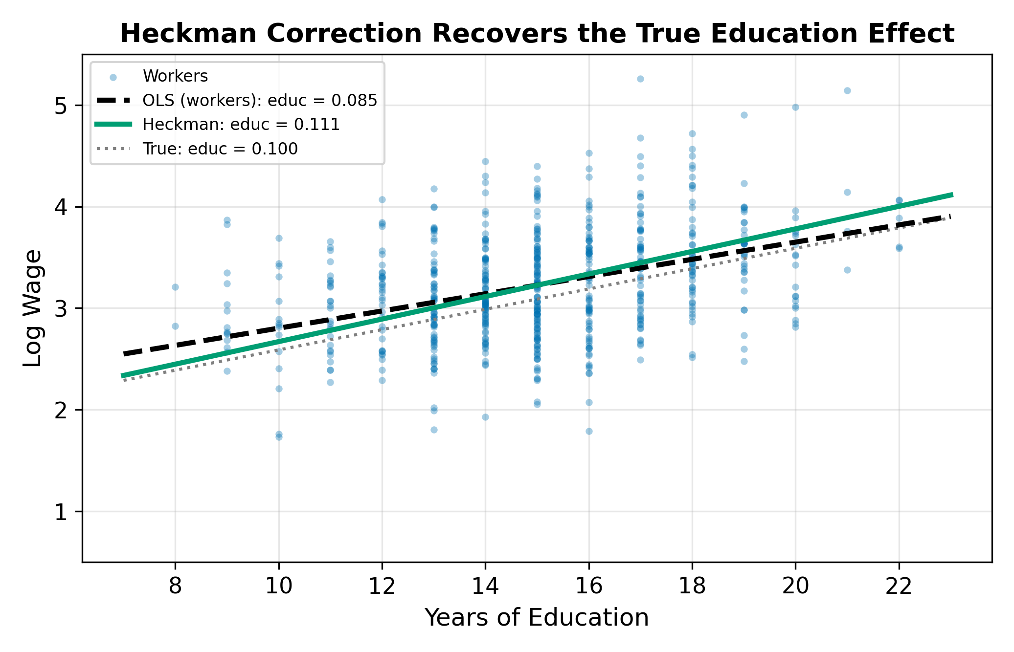
In the mroz wage data (a classic dataset in labor economics), the Heckman two-step typically yields \(\hat{\delta} > 0\), indicating positive selection. Women who participate in the labor force tend to have higher unobserved wage determinants than non-participants. Naive OLS on working women overestimates wages at each education level because the sample is drawn from the upper tail of the unobserved ability distribution.
If the \(t\)-test on \(\hat{\delta}\) fails to reject \(H_0: \delta = 0\), there is no evidence of selection bias. You can use OLS on the selected sample without the correction term. In practice, many researchers report both the OLS and Heckman estimates. If the coefficient estimates are similar and \(\hat{\delta}\) is insignificant, OLS is preferred because it is more efficient (fewer parameters to estimate, no generated-regressor problem).
20.6 Identification: The Exclusion Restriction
The Heckman model requires at least one variable that appears in the selection equation (Equation 20.2) but not in the outcome equation (Equation 20.3). In our example, \(\text{kids}\) and \(\text{spouse\_inc}\) affect the decision to work but (arguably) do not directly affect wages conditional on working. These excluded variables play the same role as instruments in IV estimation: they provide variation in the selection probability that is independent of the wage error.
Without an exclusion restriction, the model is identified only through the nonlinearity of the inverse Mills ratio. The probit produces a nonlinear function of the selection index, and it is this nonlinearity that distinguishes \(\hat{\lambda}_i\) from a linear combination of the regressors already in the wage equation. In principle, this is sufficient for identification. In practice, identification by functional form alone is fragile: if the data happen to fall in a region where \(\lambda\) is approximately linear, the correction term is nearly collinear with the regressors, and estimates become unstable.
This is the Heckman model’s Achilles heel. If you cannot find a plausible exclusion restriction, the correction rests on distributional assumptions alone. Sensitivity to the normality assumption is a well-documented concern.
The connection to IV is direct. The excluded variable provides exogenous variation in the probability of selection (relevance) without directly affecting the outcome (exogeneity). The difference is that in standard IV, the instrument enters through a linear first stage; in Heckman, it enters through a nonlinear probit first stage, which produces the inverse Mills ratio as the “generated instrument.”
Good exclusion restrictions in labor economics:
- Number of young children (\(\text{kids}\)): affects the reservation wage and hence the work decision, but should not affect the market wage offer
- Spouse’s income (\(\text{spouse\_inc}\)): affects the financial pressure to work, but should not affect the employer’s wage offer
- Local labor market conditions (unemployment rate in the county): affects whether someone can find a job, but should not affect the wage offered to a particular individual
Each of these can be challenged. Do children affect wages through reduced human capital accumulation during parental leave? Does spouse income proxy for neighborhood quality, which affects wages? The strongest exclusion restrictions are those where the economic argument for exclusion is compelling and robust to alternative channels.
\(\implies\) The credibility of the Heckman correction depends almost entirely on the plausibility of the exclusion restriction. Without it, treat the results with caution.
20.7 Heckman vs. Tobit
Both models deal with observed zeros, but they tell different stories about what generates the zero.
Tobit: A single latent variable \(y^*\) drives both the participation decision and the observed amount. The zero arises because \(y^*\) falls below the censoring point. The same process, the same parameters, and the same error term govern whether we see a positive value and how large that value is. A variable that increases the probability of a positive outcome also increases the conditional mean by a proportional amount.
Heckman: Two separate processes operate. One process (with its own error \(v\)) determines whether we observe the outcome at all. A different process (with its own error \(u\)) determines the outcome’s value conditional on observing it. The zeros are missing data, not censored data. A variable can increase the probability of participation while decreasing the conditional outcome, or vice versa.
| Feature | Tobit | Heckman |
|---|---|---|
| Number of equations | 1 | 2 |
| Number of error terms | 1 | 2 (correlated) |
| Zeros are… | Censored values (\(y^* \leq 0\)) | Missing data (outcome not observed) |
| Same parameters for selection and outcome? | Yes | No |
| Requires exclusion restriction? | No | Yes (in practice) |
| Example | Hours worked = 0 because desired hours \(\leq\) 0 | Wages missing because person chooses not to work |
The distinction is conceptual, not statistical. Ask: “Does the same mechanism produce the zero and the positive value?” If yes, Tobit. If the decision to participate and the level of the outcome are governed by different factors, Heckman.
The choice between Tobit and Heckman is a modeling decision, not a statistical test. Consider charitable donations. If you model donations as censored (people want to donate but are constrained to \(\geq 0\)), Tobit is appropriate. If you model the decision to donate and the amount donated as separate decisions influenced by different factors (e.g., religious attendance affects whether you donate, but income determines how much), Heckman is appropriate. The data alone cannot tell you which story is correct.
\(\implies\) If a researcher uses Tobit when the true data-generating process has separate selection and outcome equations, the single-equation restriction forces the wrong structure on the data and biases both the participation and the amount estimates.
Return to the Qualitative and Limited DV hub for the full chapter map, or continue to Regularization for penalized regression methods (LASSO, Ridge) that handle high-dimensional data.